Chapters
Engineer matrices and vectors
The Engineer mode has two dedicated surfaces for linear algebra: Matrix and Vector. Both work the same way - you edit numbers into a bracketed grid on the left, then press an operation button to compute a result, which appears as a card below. Nothing is typed as an expression here; you fill cells and click. You reach both from the app rail down the left edge of the Engineer window: the Matrix tile and the Vector tile, which sit between CAS and Units. This chapter covers the two surfaces in turn.
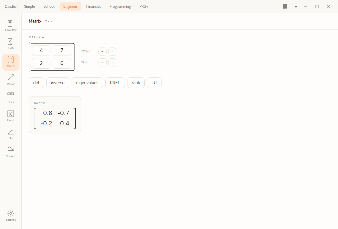
Across the top of the window are the mode tabs (Simple, School, Engineer, Financial, Programming, PRG+); down the left is the Engineer app rail (Calculate, CAS, Matrix, Vector, Units, Const, Plot, Numeric, and Settings at the foot). The rest of the window is the working area for the selected surface. For the rest of Engineer mode, see the Engineer calculator.
Matrices
Open the Matrix tile from the rail. The surface has three parts stacked down the working area: the matrix editor (labelled MATRIX A) with its dimension steppers, a row of operation buttons, and the result cards the last operation produced. The header beside the word Matrix shows the current size, for example 2 x 2.
The surface holds a single matrix, A. There is no second matrix and no named-matrix store, so the operations here all act on A alone - this surface is for the single-matrix computations (determinant, inverse, and the rest), not for adding or multiplying two matrices together.
Sizing the matrix. To the right of the grid are two stepper pairs: ROWS with − and +, and COLS with − and +. Each press adds or removes one row or column. A matrix can be from 1 x 1 up to 6 x 6. The header size caption updates as you step. Changing either dimension resets every cell to 0 and clears any result already on screen, so set the size you want first, then fill in the numbers.
Entering entries. The grid is drawn inside square brackets, one editable box per entry, laid out row by row. Click a cell and type its value; use a decimal point for fractional entries (for example 1.5) and a leading minus for negatives (-2). When the surface first opens it is seeded with a worked 2 x 2 example, [[4, 7], [2, 6]], so you have something to compute against immediately. If a cell is left blank or holds something that is not a number, the operation stops and a status line tells you which cell is at fault, for example Cell [1,2] is not a number.
The operations. Below the editor is one button per operation. These are the only matrix operations the surface offers:
| Button | What it computes | Result shape | Needs a square matrix |
|---|---|---|---|
det |
The determinant of the matrix. | A single number | Yes |
inverse |
The inverse matrix (the matrix that undoes A). |
A matrix | Yes |
eigenvalues |
The eigenvalues of the matrix. | A list of numbers | Yes |
RREF |
The reduced row-echelon form (full row reduction). | A matrix | No |
rank |
The rank - how many rows are genuinely independent. | A single number | No |
LU |
The LU decomposition, returned as three matrices L, U, and P. |
Three matrices | Yes |
det, inverse, eigenvalues, and LU are defined only for a square matrix; while the matrix is non-square those four buttons are dimmed, and hovering one explains Requires a square matrix. RREF and rank work on any shape and stay available.
Reading the results. Each operation replaces the cards below. A single-number result (det, rank) shows as a large accent value under its operation label. A matrix result (inverse, RREF) shows as a bracketed grid. eigenvalues lists its values side by side, and shows a complex eigenvalue in a + bi form when one arises. LU produces three separate cards, L, U, and P. If an operation cannot be done - asking for the inverse of a singular matrix, for instance - no card appears and the status line explains why, such as The matrix is singular (no inverse).
Worked example - invert a 2 x 2. Using the seeded matrix [[4, 7], [2, 6]]:
-
Confirm the header reads
2 x 2and the cells hold4,7,2,6. -
Press
det. The result card shows10- the determinant is non-zero, so the matrix has an inverse. -
Press
inverse. The card shows the bracketed grid[ 0.6 -0.7 ] [ -0.2 0.4 ]
That is (1 / 10) times [[6, -7], [-2, 4]], exactly as the closed form for a 2 x 2 inverse predicts. To check the inverse yourself, multiply it back against A by hand; the product is the identity matrix. For the mathematics behind these operations, see Matrices.
Vectors
Open the Vector tile from the rail. This surface works in three dimensions: the header reads Vector · 3-space, and it holds two vectors, A and B, each with three components.
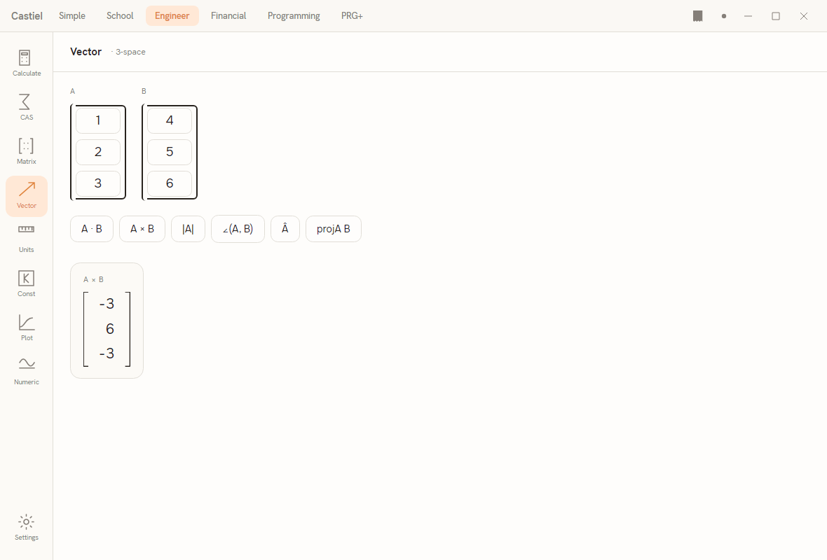
Entering a vector. Each vector is a bracketed column of three editable boxes - the x, y, and z components from top to bottom. Click a box and type; decimals and negatives are accepted, just as in the matrix editor. The surface opens seeded with A = (1, 2, 3) and B = (4, 5, 6). If a component is blank or non-numeric, the operation stops and the status line names the offending vector and component, for example Vector A: y is not a number.
The operations. The buttons below the two columns are the only vector operations offered:
| Button | What it computes | Uses | Result shape |
|---|---|---|---|
A · B |
The dot product of A and B. |
Both | A single number |
A × B |
The cross product of A and B - a vector perpendicular to both. |
Both | A vector |
|A| |
The magnitude (length) of A. |
A only |
A single number |
∠(A, B) |
The angle between A and B. |
Both | A single number |
 |
The unit vector of A - A scaled to length 1, keeping its direction. |
A only |
A vector |
proj_A B |
The projection of B onto A - the part of B that lies along A. |
Both | A vector |
Two of these, |A| and Â, read only the first vector A; the other four read both. A single-number result shows as a large accent value under the operation label; a vector result shows as a bracketed column of three components.
Worked example - cross product of two 3-vectors. Using the seeded vectors A = (1, 2, 3) and B = (4, 5, 6):
-
Confirm column
Aholds1,2,3and columnBholds4,5,6. -
Press
A × B. The result card shows the bracketed column[ -3 ] [ 6 ] [ -3 ]
That is the cross product A × B = (2·6 − 3·5, 3·4 − 1·6, 1·5 − 2·4) = (−3, 6, −3). The result is perpendicular to both inputs, which you can confirm by pressing A · B and checking the dot product against it. As a second pass, press A · B on the original vectors to get 32, and |A| to get the length of A (the square root of 1 + 4 + 9). For the mathematics behind these operations, see Vectors.
Related chapters
- The Engineer calculator - the rest of Engineer mode and its app rail.
- Matrices - determinants, inverses, and row reduction explained.
- Vectors - dot and cross products, magnitude, and projection explained.