Chapters
The School 3D graph
The 3D graph is where School mode plots surfaces. Where the ordinary Graph draws a curve y = f(x) on a flat plane, the 3D graph draws a surface z = f(x, y) in space: a landscape whose height at each point on the floor is given by your formula. You reach it from the 3D Graph tile on the left apps rail, one tile below Graph.
Use it whenever a quantity depends on two inputs at once - a saddle x² − y², a ripple sin(xy), a paraboloid x² + y² - and you want to see its shape, turn it over, and read heights off it. Alongside surfaces you can drop in a few built-in solid shapes (a line, a plane, a sphere, a cylinder) to mark or frame what the surface is doing. For single-variable plotting, statistics, or equations, use the matching tile instead; see the School apps for the full set.
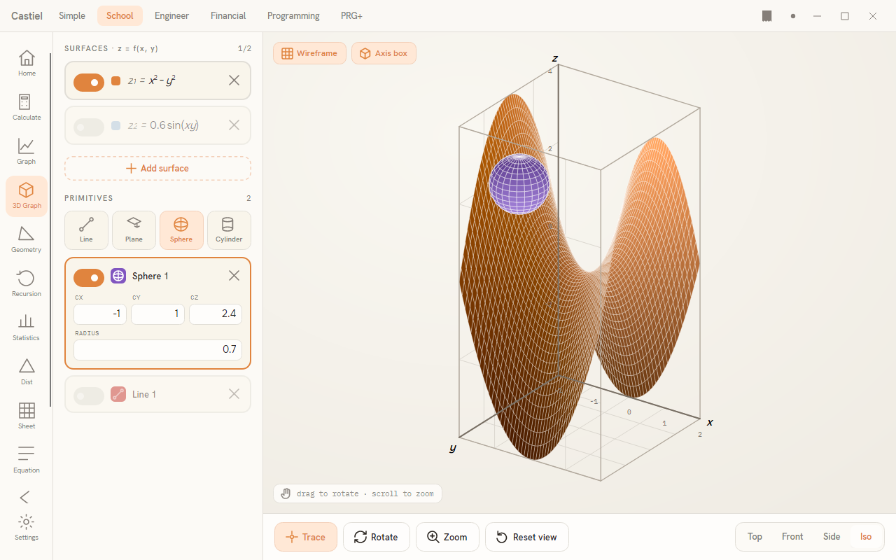
The window has two parts. Down the left edge is the entry rail, a scrollable column with two stacked panels: SURFACES at the top (your z = f(x, y) formulas) and PRIMITIVES below (the built-in shapes). Filling the rest of the window is the render area, where the surface is drawn in 3D. Floating controls sit in its corners, and a view toolbar runs across the bottom.
The render area
The centre of the surface sits on a shaded floor with a faint radial grid; a wireframe box (the axis box) frames the region being plotted. The surface itself is drawn as a shaded mesh, higher parts of it tinted toward the surface's colour so you can read height at a glance.
Two floating controls sit in the corners:
- Top-left - the display chips.
Wireframeoverlays the mesh grid lines on the surface;Axis boxshows or hides the framing box. Each is a latch: tap to turn it on (it highlights), tap again to turn it off. In the screenshot both are on. - Bottom-left - the movement hint. A small reminder that reads
drag to rotate · scroll to zoom- the two gestures you use most. - Top-right - the trace readout. A card that appears once you are tracing a surface, showing the exact coordinates of the point under the tracer (covered under Reading a surface below).
Turning the surface over. The most useful thing you can do with a 3D plot is look at it from another side. Drag inside the render area to orbit the camera around the surface; scroll (or pinch) to zoom in and out. The surface stays put - you are moving your viewpoint around it. Turn it until the feature you care about faces you.
The view toolbar
The strip across the bottom sets how you move the camera and which fixed viewpoint you are looking from.
On the left - the movement tools and reset.
| Tool | What a drag in the render area does |
|---|---|
Trace |
Runs a tracer over the nearest surface and reports the point's coordinates in the readout card. |
Rotate |
Orbits the camera around the surface. |
Zoom |
Drags the camera closer or further. |
Reset view |
Returns the camera to the default three-quarter framing (orientation and distance), leaving your surfaces and shapes untouched. |
Trace, Rotate, and Zoom are a one-of-three choice - the active tool is highlighted. Reset view is a one-shot button, not a mode. Note that a drag rotates and the scroll wheel zooms whichever tool is selected; the tool chiefly decides what a drag does.
On the right - the orientation presets. A four-way segmented control snaps the camera to a fixed viewpoint:
| Preset | What you see |
|---|---|
Top |
Looking straight down, as if the surface were a contour map on the floor. |
Front |
A near-level view from the front - a slim, side-on silhouette of the surface. |
Side |
The same slim silhouette seen from the side. |
Iso |
The default three-quarter (isometric) view, the one the surface opens on. |
The highlighted preset is the one the camera currently sits on. As soon as you drag the view off it, the highlight clears - you are now on a free angle. Tap any preset to snap back, or Iso to return to the opening view.
Entering a surface
The SURFACES panel lists your formulas, one per row. Its header reads SURFACES · z = f(x, y), and a small count on the right shows how many are switched on out of the total - 1/2 means two rows exist and one is currently drawn.
Each row has four parts, left to right: a switch that draws or hides the surface, a colour swatch that keys the surface to its colour in the render area, the label z1 = (z2 =, z3 =, and so on), and its formula. A small × at the right of the row deletes it.
To type or change a formula, select its row first. Tap a row and its formula turns into an editable field; type the right-hand side of z = ... using x and y as the two variables. The surface re-plots as you type - there is no execute key to press. Tap another row (or an empty part of the rail) and the formula settles back into clean typeset notation.
To add another surface, tap the dashed Add surface button under the list; a fresh empty row appears ready for a formula. When you first open the 3D graph, the top row is already filled with the classic saddle z1 = x² − y², so there is always something to look at.
Worked example - plot a saddle and inspect it.
- Open the 3D graph from the 3D Graph tile. The saddle
z1 = x² − y²is already plotted in the default three-quarter view. - Drag inside the render area to orbit. Turn the surface until you can see its shape clearly: it rises along one diagonal and falls along the other, like a Pringle or a mountain pass. Scroll to zoom in.
- Tap
Topon the right of the toolbar to look straight down - from above, the rising and falling directions read like a contour map. TapIsoto return to the three-quarter view. - To try a different surface, tap the
z1row and change the formula tox^2 + y^2. The saddle becomes a smooth bowl (a paraboloid) the moment you finish typing. TapReset viewif you want the framing back to the default.
Plotting several surfaces at once
You can show more than one surface together to compare them or watch where they meet. Tap Add surface, select the new row, and type a second formula - for example z2 = 0.6 sin(x y) alongside the saddle. Each surface is drawn in its own colour, matched to the swatch on its row, so you can always tell which mesh is which. The rail's count updates to reflect how many are switched on.
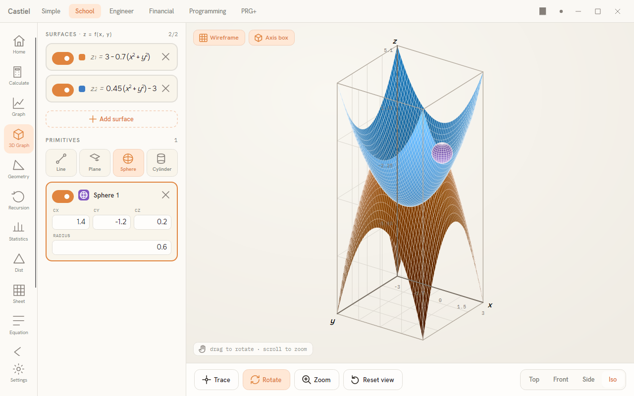
The row switch is the quick way to declutter: turn a surface off and it drops out of the render area and out of the count, but stays in the list with its formula intact, ready to switch back on. Deleting a row (the ×) removes it for good and renumbers the rest so the labels stay z1, z2, z3 in order.
A note on trig and angle units. A formula such as sin(x y) uses the same trigonometric functions as the rest of School, and they read the calculator's angle mode (RAD, DEG, or GRA) set in Settings - the same setting that governs the School calculator. The 3D graph has no angle indicator of its own, so if a surface with a sin or cos in it looks unexpectedly stretched or compressed, check the angle mode in Settings. See trigonometry for what the mode changes.
Built-in shapes
The PRIMITIVES panel adds simple solid shapes to the scene - useful for marking a point, a direction, or a boundary against your surface. Four kinds are available, chosen from the row of buttons at the top of the panel:
| Shape | What it is | The numbers you give it |
|---|---|---|
Line |
A straight segment between two points. | Start point A and end point B, each as x, y, z. |
Plane |
A flat panel floating in space. | A point P on it, a normal direction N it faces, and a size. |
Sphere |
A ball. | Its centre C as x, y, z, and a radius. |
Cylinder |
A tube or rod. | A base centre, an axis direction, a radius, and a height. |
Tapping one of the four buttons does two things at once: it places a shape of that kind into the scene with sensible starting numbers, and it selects the new row so its settings open up. The panel header keeps a count of how many shapes you have placed.
Each placed shape gets its own row with a switch (show or hide it), a coloured kind icon, a name that numbers each kind on its own - Sphere 1, Sphere 2, Line 1 - and a × to remove it. Select a row to reveal its settings: a small grid of numeric fields, one set per kind, where you type the coordinates and sizes from the table above. Edit any field and the shape updates immediately. In the opening screenshot, a violet Sphere 1 is selected and resting on one ridge of the saddle, with its centre and radius fields showing.
Reading a surface
To read exact values off a surface rather than just eyeing its shape, use the Trace tool. Select Trace in the bottom toolbar, then run the tracer over the surface; the calculator finds the nearest plotted point and shows the trace readout card in the top-right corner.
The card names the surface being traced (TRACE · z1) with a colour swatch matching that surface, then lists the point's three coordinates stacked:
xandy- where you are on the floor;z- the surface's height there, shown in the surface's accent colour.
The z value is a genuine evaluation of your formula at that x and y, so tracing is the way to answer "how high is the surface at this spot?" without reading it off the picture by eye. Whole numbers show without a decimal point; other values show to several decimal places.
Related chapters
- The School graph - plotting single-variable curves
y = f(x), the 2D sibling of this surface. - The School calculator - everyday evaluation, and where the angle mode is explained.
- Trigonometry - the
sin,cos, andtanfunctions you can use inside a surface formula. - The School apps - Graph, Statistics, Equation, and the rest of the rail.