The Engineer numeric solver

The numeric solver is where Engineer mode finds a root of an equation by iteration — the value of x that makes an expression equal zero. You reach it from the Numeric tile on the Engineer apps rail, or with the Ctrl/Cmd + Shift + N shortcut. It uses the Newton-Raphson method: you give it a function and a starting guess, and it steps towards a root, showing you every step it took and how close it got.

Use the numeric solver when an equation has no tidy closed-form answer, or when you would rather have a decimal root to a stated accuracy than a symbolic expression. It is the numerical counterpart to the CAS surface: CAS solves symbolically and returns exact forms where they exist; the numeric solver solves by approximation and works on almost any function you can write, including ones with no exact solution at all.

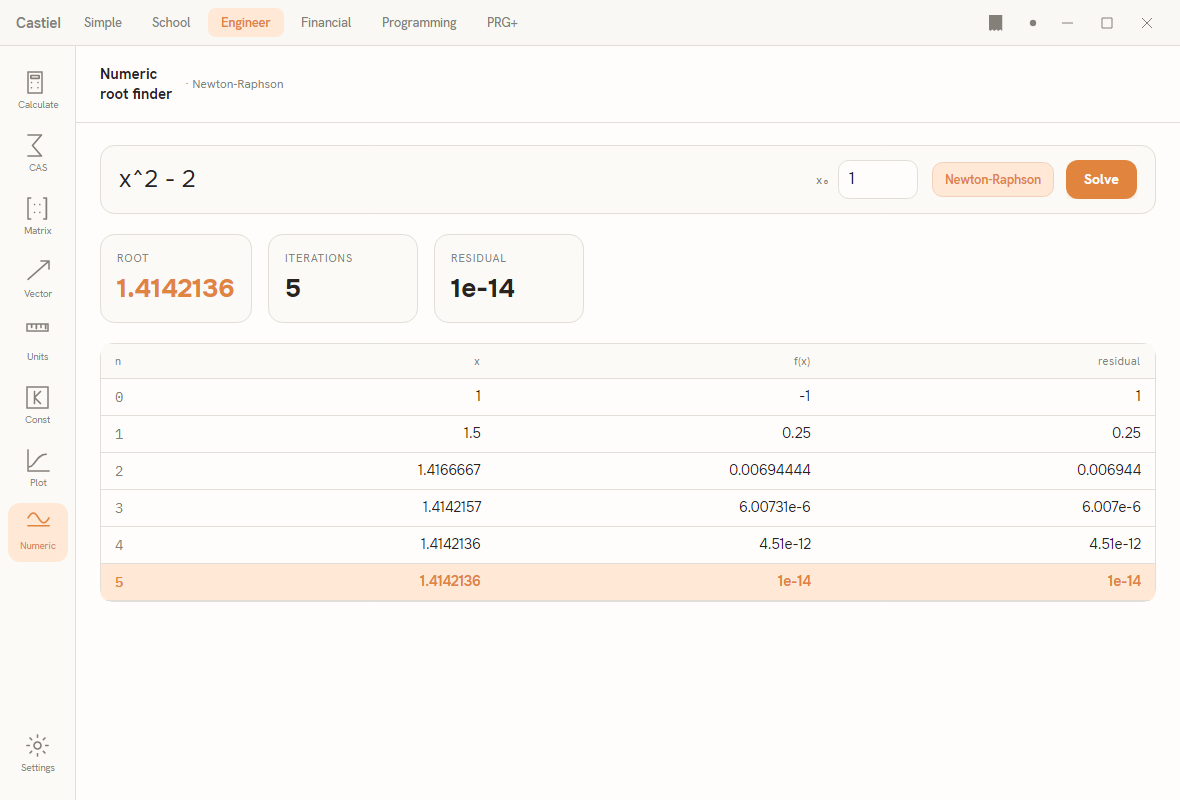
The surface has three parts stacked down the panel. At the top is the equation row: a wide field for the function f(x), a small box for the initial guess x₀, the method segment (fixed to Newton-Raphson), and the Solve button. Below it, once you solve, sits a row of three result cards — ROOT, ITERATIONS, and RESIDUAL. Beneath those is the iteration trace table, which lists every step the method took. A status line appears between the cards and the table when there is something to report — a typing error in the equation, or a warning that the method did not settle.

Setting up a solve

The equation. Type the function into the wide f(x) field. You are entering the expression that should equal zero: the placeholder f(x), e.g. x^2 - 2 means "solve x² − 2 = 0". Write it in ordinary linear form — ^ for a power, * for a multiplication, parentheses for grouping — using the same function names the rest of the calculator accepts (sin, cos, ln, sqrt, and so on). If your problem is stated as two sides that should be equal, g(x) = h(x), rearrange it to one side equal to zero and enter g(x) - h(x).

The initial guess. The x₀ box holds the starting point. Newton-Raphson begins at your guess and refines it; the closer your guess is to the root you want, the fewer steps it takes and the more reliably it lands on the root you had in mind. A function can have several roots, and the method converges to the one nearest the path it follows from x₀ — so the guess is how you choose which root you get. If you leave the box blank or type something that is not a number, the solver falls back to a guess of 1.

The method. The method segment shows Newton-Raphson and is fixed: it is the one method this surface offers. Newton-Raphson uses the slope of the function at each point to jump towards the root, which makes it fast when it works — well-behaved problems converge in a handful of steps.

Press Solve (the surface also solves once on opening, seeded with the x² − 2 example, so you always see a worked result to read). The result cards and the trace table fill in.

Reading the result

The result cards. Three cards summarise the outcome:

The residual is your quality check. A numeric root is an approximation, so f(root) will rarely be exactly zero; the residual tells you how close it came. If the residual is tiny, trust the root. If it is not small, the method stopped early or wandered — read the status line and the trace to see what happened.

The iteration trace. The table below the cards shows the whole journey, one row per step:

Reading down the residual column tells the story: the numbers should shrink rapidly towards zero as the estimates home in on the root. The converged row — the final, accepted step — is highlighted in the accent colour so you can see at a glance where the method stopped. Watching the trace is instructive in its own right: it shows how Newton-Raphson works, doubling the number of correct digits at each step once it is close.

When it does not converge

Newton-Raphson is fast but not guaranteed. It can fail to settle — a poor starting guess, a function whose slope flattens out, or a root that the method keeps overshooting. The solver protects you in three ways:

• A typing error in the equation stops the solve before it starts. The status line explains the problem (for example, a prompt to enter an equation in x when the field is empty), and the cards stay blank. Fix the expression and press Solve again.
• Non-convergence — the method ran its full budget of steps without meeting the accuracy target — still gives you an answer. The status line reads that Newton-Raphson did not converge within the iteration limit and that the best estimate so far is being shown. The cards and trace are filled in with that best estimate, so you can judge it yourself from the residual and decide whether to try a different starting guess.
• A breakdown — the step running off to infinity or an undefined value — ends the run and reports the last usable estimate rather than a meaningless number.

If a solve does not converge, the usual fix is a better x₀: pick a value closer to where you expect the root, and the method will follow a cleaner path to it. Plotting the function first (on the Engineer plot surface) is a good way to see roughly where the roots are before you guess.

Numeric versus exact: choosing this surface or CAS

The numeric solver and the CAS surface answer the same kind of question — "what value of x solves this?" — in opposite ways, and knowing which to reach for saves time.

• CAS solves symbolically. It manipulates the equation with algebra and returns an exact result where one exists: a fraction, a radical such as √2, a multiple of π, or every root of a polynomial at once. When a closed form exists, CAS gives you the truest possible answer. But many equations have no closed form, and for those CAS cannot help.
• The numeric solver approximates. It ignores the algebra and hunts for the root by stepping towards it from your guess, returning a decimal to a fixed accuracy. It does not care whether a closed form exists — it works on transcendental equations, mixtures of functions, and anything else you can write. In exchange, it finds one root at a time (the one near your guess), and its answer is an approximation with a residual, not an exact expression.

A concrete contrast: solving x² − 2 = 0 in CAS returns the exact √2; solving it here returns 1.4142136 with a near-zero residual. Both are correct — one is the symbol, one is its decimal value. Reach for CAS when you want the exact form and the equation is tractable; reach for the numeric solver when the equation is messy, when no closed form exists, or when a decimal to a known accuracy is all you need.

What this surface does not cover. The numeric solver finds roots only. Numerical integration and differentiation live elsewhere: enter a definite integral or a derivative with the ∫ and d/dx templates on the calculator keypad (see Calculus basics), or ask CAS to integrate or differentiate symbolically. For solving a standalone equation without the iteration trace — including linear and quadratic equations with all their roots at once — the equation solver is often the simpler tool.

Worked examples

Example 1 — a square root by iteration. Find √2 by solving x² − 2 = 0. This is the example the surface opens with.

1. In the f(x) field type x^2 - 2.
2. In the x₀ box type 1.
3. Press Solve.

The ROOT card reads 1.4142136, the decimal value of √2. The ITERATIONS card shows a small count — Newton-Raphson reaches full accuracy here in about five steps — and the RESIDUAL card shows a value near zero, confirming the root is good. In the trace, row 0 is your guess 1 (with residual 1, since f(1) = −1); each following row roughly doubles the number of correct digits — 1.5, then 1.4166…, then 1.4142157…, then the highlighted converged row at 1.4142136. Compare this with CAS, which would return the exact √2 for the same equation.

Example 2 — a root with no tidy form. Find a real root of x³ − x − 2 = 0. This cubic has one real root, and it is not a friendly number, which is exactly the case the numeric solver is built for.

1. Type x^3 - x - 2 into the f(x) field.
2. Type 1 into the x₀ box.
3. Press Solve.

The ROOT card reads about 1.5213797, with a residual near zero. Newton-Raphson steps out from 1 and closes in on the root over a few iterations, each shrinking the residual, until the highlighted converged row. Asked to solve the same cubic, CAS would return an exact but unwieldy nested-radical expression; the numeric solver gives you the decimal you can actually use — and, in the trace, the confidence of watching the residual fall to zero.

The pattern is the same in both examples: write f(x), choose a starting guess near the root you want, solve, then read the root from the card and confirm it with the residual and the trace.

Related chapters

• The Engineer calculator — the mode overview and the other Engineer surfaces (plot, matrix, units, constants).
• CAS — symbolic solving, integration, and differentiation for exact answers.
• The equation solver — solving standalone linear, quadratic, and system equations with all roots at once.
• Calculus basics — definite integrals and derivatives with the ∫ and d/dx templates.