Chapters
The School spreadsheet
The School spreadsheet - "Sheet" on the apps rail - is a full cell grid built into School mode. You reach it from the Sheet tile on the left rail. Use it whenever your work is a table rather than a single expression: a set of exam marks to average, a list of measurements to chart, a column of function values to generate, or data you have pasted in from a file. It is deliberately richer than the small spreadsheet found on a graphing calculator: it charts, it formats cells by their values, it holds several sheets in one workbook, and it reads and writes CSV.
For a single calculation, the School calculator is the better surface; for statistical summaries and distributions, see Statistics. The spreadsheet complements both - you build a table here, then feed it to those surfaces. See the School apps for the whole rail.
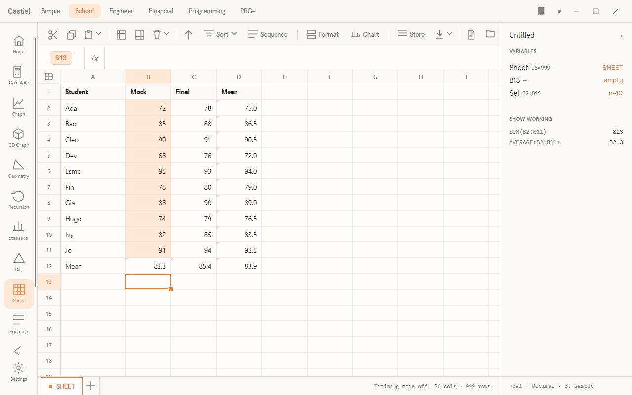
The window has three horizontal bands above the grid and one below it. Across the top is the toolbar, a row of icon buttons grouped by task (clipboard, structure, data, format and chart, file and CSV) with a Training switch at its right end. Beneath it is the formula bar: an address pill on the left, an fx marker, then the contents of the selected cell. The grid itself fills the centre, columns lettered A, B, C… across the top and rows numbered 1, 2, 3… down the side. Along the bottom is the sheet-tab strip, one tab per sheet plus a + to add another. A Variables / Show working panel runs down the right edge, mirroring the active cell and the current selection into a live readout.
Entering data and formulas
Click any cell to select it; its address (for example B2) appears in the pill at the left of the formula bar. Start typing to enter content, and press EXE (or Enter) to commit it and move down. What you type falls into three kinds:
- A number or literal -
72,3.14,-5. Stored and shown as a value. - Text - a heading such as
StudentorMark. Text in row 1 is treated as a bold header row for the column beneath it. - A formula - anything beginning with
=. The cell shows the computed result; the formula itself stays visible in the formula bar whenever the cell is selected.
Cell references. Inside a formula, refer to another cell by its address: =A1+A2 adds the two cells above. A rectangular block of cells is a range, written as its top-left and bottom-right corners joined by a colon - A1:A10 is the first ten cells of column A, and B2:D5 is a block three columns wide and four rows tall. Most built-in functions take a range: =SUM(A1:A10) adds that whole column.
The formula bar. The formula bar always reflects the selected cell. Click into it (or press EXE on a cell) to edit; the contents are colour-coded as you type, with the leading = and cell references picked out so a long formula stays readable. A blinking caret marks where your typing lands. Press EXE to commit, or Esc to abandon the edit and leave the cell as it was.
Picking references by clicking. While you are editing a formula that starts with =, clicking or dragging across cells in the grid inserts their address or range into the formula instead of moving the selection. This lets you point at A1:A10 rather than type it.
The function helper. As you type a function name into a formula, a small popover lists the matching functions with a one-line description of each - for example SUM(range) — add all the values in a range. Use the up and down arrows to choose one and press Tab to insert it (with its opening parenthesis). The popover footer counts how many functions match what you have typed so far. If a formula names a function the spreadsheet does not recognise, the cell shows an error and, for a misspelling, suggests the closest real name ("Did you mean AVERAGE? Press Tab to accept").
Built-in functions
The spreadsheet ships with a broad library of functions, grouped by purpose. You do not need to memorise them - the function helper lists and describes them as you type - but it is worth knowing the categories so you know what is available:
| Category | What it covers | Examples |
|---|---|---|
| Aggregates | Combine a range into one value | SUM, AVERAGE (also MEAN), MEDIAN, MIN, MAX, PRODUCT |
| Counts | Count cells that qualify | COUNT, COUNTA, COUNTBLANK, COUNTIF |
| Spread | Standard deviation and variance | STDEV, STDEVP, VAR, VARP |
| Rounding and number | Reshape a number | ROUND, ROUNDUP, ROUNDDOWN, TRUNC, FLOOR, CEILING, ABS, SQRT, POWER, INT, MOD |
| Logic | Combine true/false tests | AND, OR, NOT |
| Descriptive extras | Order statistics | MODE, QUARTILE, RANK, LARGE, SMALL |
| Conditional aggregates | Aggregate only what passes a test | SUMIF, AVERAGEIF, SUMPRODUCT |
| Lookup | Find a value in a range | LOOKUP |
| Text | Work with text | LEN, LEFT, RIGHT, MID, CONCAT, TRIM, UPPER, LOWER |
| Regression | Line-of-best-fit measures | CORREL, SLOPE, INTERCEPT, RSQ |
The Spread category makes the sample-versus-population distinction explicit: STDEV and VAR divide by n − 1 (the sample forms), while STDEVP and VARP divide by n (the population forms). Choose deliberately - for GCSE and A-Level work the population σ is usually what is expected.
The row and column context menu
Right-click a cell to open its context menu - the fastest route to the structure and clipboard actions.
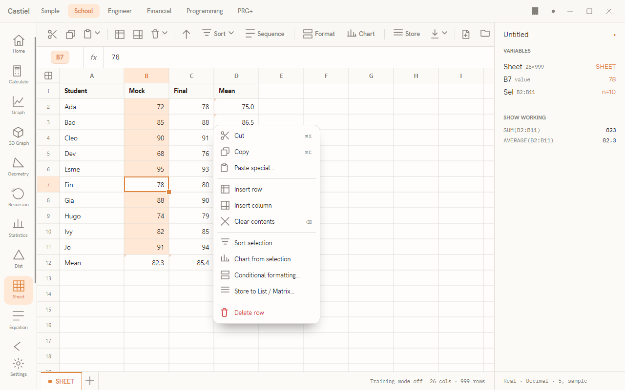
The menu offers Cut, Copy and Paste special…, then Insert row and Insert column (which push existing cells down or right), Clear contents (empties the cell but keeps the row and column), Sort selection, Chart from selection, Conditional formatting…, Store to List / Matrix…, and a Delete row at the foot. The same clipboard and structure actions live in the toolbar's first two groups; the toolbar's Delete button additionally carries a small dropdown with Delete row, Delete column, Clear contents and Delete all.
When you cut or copy a range and paste it elsewhere, references inside the pasted formulas are rewritten to match their new position. Paste special (in the toolbar's clipboard group, or from the context menu) lets you paste Values only, Formulas only, or Transpose (swap rows and columns) instead of a plain paste.
Charts
Select a column of numbers (or two columns) and choose Chart from the toolbar, or Chart from selection from the context menu. A chart pane opens to the right of the grid. The chart type is offered according to the shape of your selection:
- One column of values can be drawn as a Histogram, a Box plot, or a Bar chart.
- Two columns - an x column and a y column - can be drawn as a Scatter plot or an XY-Line.
Pick the type from the chips at the top of the pane. A header row (text in row 1) is recognised and left out of the plotted data automatically.
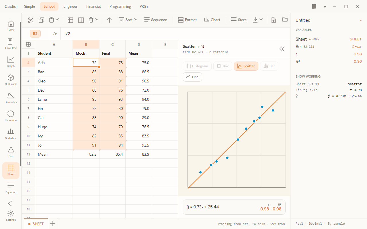
For a histogram, a stepper at the foot of the pane sets the number of bins, and the read-out shows the data range, the count n, and the modal bin. For a scatter plot, the spreadsheet draws the line of best fit through the points and reports the fit's equation together with the correlation r and the coefficient of determination R². The chart is live: edit any source cell and the plot redraws. (With Training mode on, the scatter fit is held back until you ask for it, so you can estimate the line by eye first - see the note on Training below.)
Conditional formatting
Conditional formatting colours cells by their values, so a pattern in a column jumps out. Open it with the Format button on the toolbar, or Conditional formatting… from the context menu; a rules panel docks to the right of the grid.
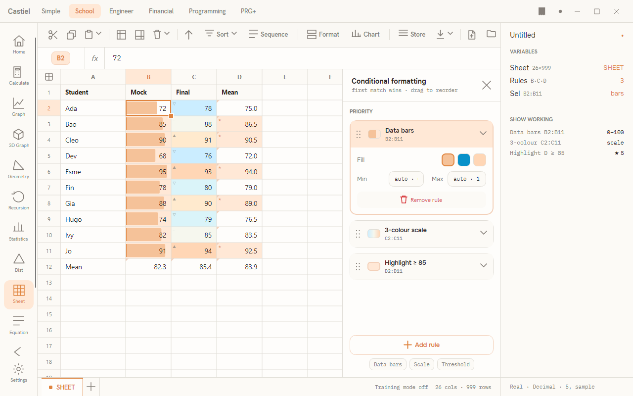
Add a rule with Add rule and pick one of three kinds:
- Data bars - draw a proportional bar inside each cell, longest for the largest value.
- Scale - shade cells along a colour gradient from low to high.
- Threshold - flag cells that cross a value you set.
Rules are listed in priority order, and the first rule that matches a cell wins; drag a rule by its grip to reorder. Expand a rule to edit its fill colour and its minimum and maximum, and remove it with Remove rule. While the panel is open with rules active, the sheet-tab meta reads "N rules active".
Multiple sheets
A spreadsheet document is a workbook that can hold several sheets, each its own grid. The tabs along the bottom of the window are the sheets; the active one carries an accent edge and accent text.
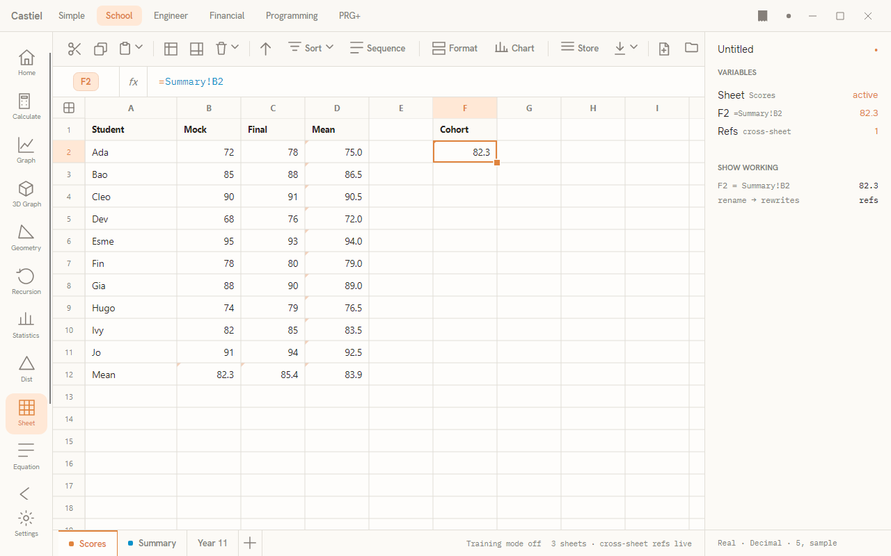
- Add a sheet with the
+button at the end of the tab strip. - Switch sheets by clicking a tab.
- Rename a sheet by double-clicking its tab and typing a new name.
- Reorder sheets by dragging a tab.
- Delete a sheet by right-clicking its tab. Because a formula on one sheet can reference another, deleting a sheet is confirmed first: any formula elsewhere that pointed into the deleted sheet becomes a
#REFerror.
CSV import and export
CSV (comma-separated values) is the common exchange format for tabular data, readable by every spreadsheet and many instruments. The CSV button on the toolbar carries a dropdown with Import CSV… and Export to clipboard.
Import opens a dialog where you set whether the first row is a header, choose the delimiter (Comma, Tab, or semicolon), and name the cell to paste the data into. A preview shows the first few rows before you commit. Import writes the table into the grid at the anchor cell.
Export copies the current selection (or the whole used area of the sheet, when only one cell is selected) out as CSV text using the chosen delimiter.
Fraction display
Where a cell's value is an exact fraction - the result of =1/3, or a sum that lands on a rational value - the spreadsheet can show it stacked as a fraction rather than as a decimal. When the selected cell holds such a value, an S⇔D pill appears at the right of the formula bar. Toggle it to flip that cell between its exact fraction and its decimal approximation; the underlying value never changes, only how it is shown. The right-hand panel lists both forms together, the exact fraction tagged exact and its decimal tagged decimal, so you can read the two side by side.
Generating a sequence, and storing data for other apps
Two toolbar tools connect the spreadsheet to the wider School toolkit.
Sequence (in the data group) fills a column with the values of a function. Enter an expression f(x), name the variable, give a Start, End and Step, and the cell to fill from; the dialog previews the column it will generate before you commit. This is the quick way to lay down a table of x and f(x) values to chart or to inspect.
Store (in the file group, or Store to List / Matrix… in the context menu) saves the current selection into a shared variable that the rest of School mode can read. Choose to store it as a List (a one-dimensional vector, the form Statistics reads), a Vector, a Matrix (reshaped as rows × columns), or a single named Alpha value. Once stored under a name, that data is recallable elsewhere - including back in a formula, =List 1.
Calling a saved sequence as a function. A sequence you have authored and saved in Castiel can be called from a cell just like a built-in function. If you have a sequence named MySeq, a formula such as =MySeq(A1) runs it with the value of A1 as its input and places the result in the cell. This turns your own saved routines into reusable spreadsheet functions. For how to write and save sequences, see Sequences as functions.
The Variables and Show working panel
The panel down the right edge tracks what you are doing. It names the active sheet and its size, echoes the active cell's value (or its exact/decimal pair, or its error code), and - when you have a range selected - reports how many numeric cells it holds and shows a small Show working tape with the SUM and AVERAGE of the selection. The document's name sits at the top with a dot marker when there are unsaved changes; the surface auto-saves in the background so a crash never loses your work, and offers to recover any auto-saved spreadsheets when you return.
The Training switch at the top-right of the toolbar turns on a teaching layer for classroom use: it prompts you to choose between sample and population standard deviation, holds back a scatter's line of best fit until you compute it, points out when a displayed decimal differs from the exact value behind it, and can trace which cells feed a formula and which depend on it.
Worked example: average a column and chart it
A short end-to-end pass, starting from an empty sheet:
- In
A1typeMarkand pressEXE. This is the column header. - Type a mark into each of
A2down toA6- say72,85,64,90,78- pressingEXEafter each. - Select
A7, type=AVERAGE(A2:A6)and pressEXE. As you type=AVthe function helper offersAVERAGE; pressTabto insert it, then fill in the range. The cell shows the mean,77.8. - Select the marks by dragging from
A2toA6, then press Chart on the toolbar. With one column selected, choose the Histogram chip; the pane draws the distribution and reports the count and modal bin. Adjust the bin stepper to regroup the bars.
Your table, its average, and its chart now all sit in one sheet - and the marks are one Store away from feeding the Statistics surface.
Related chapters
- The School calculator - the single-expression workspace alongside this one.
- Statistics - summaries and distributions over a stored list.
- Sequences as functions - writing the sequences you can call from a cell.
- The School apps - the full rail of School surfaces.
- File types - how spreadsheets and other documents are saved.