The School probability simulation

The Probability Simulation is Castiel's hands-on laboratory for chance. You reach it from the apps rail in School mode. Instead of computing a single probability, you run a random experiment thousands of times over and watch the observed results settle toward the theory. It is the surface to reach for when you want to see, rather than assert, that a fair die lands on each face one time in six, that a biased spinner favours its wide sectors, or that the average of many samples clusters into a bell curve.

Pick an experiment, shape it with a few steppers and drop-downs, then pour trials into it. The chart redraws as the counts climb, and a comparison table keeps the observed relative frequency beside the exact theoretical value so you can watch the gap close. If you want the probability of a single expression evaluated directly rather than estimated, use the School calculator; for fitting and summarising data you already have, use Statistics and Distributions.

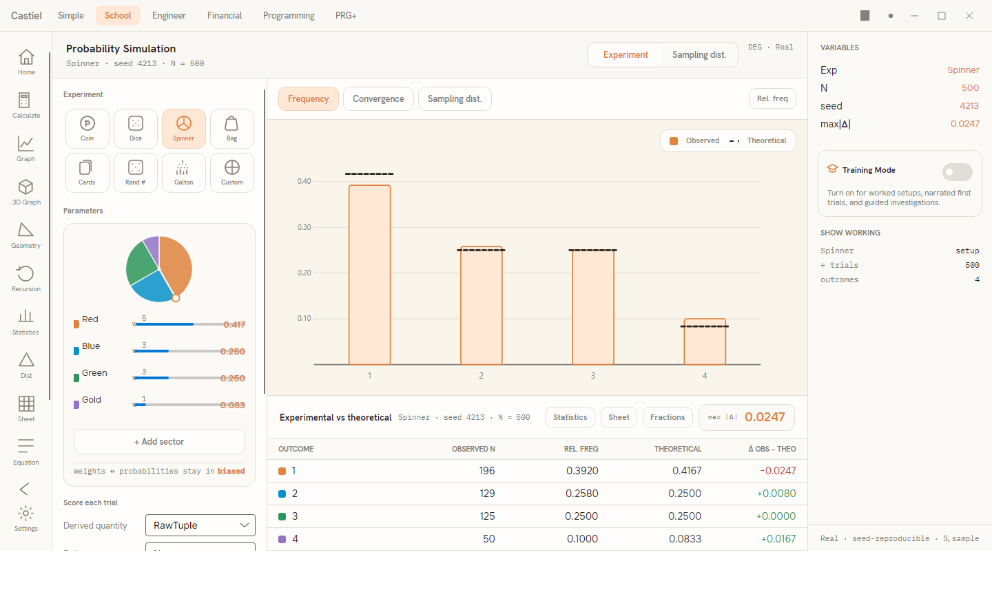
The window has three columns. The setup column on the left is where you build the experiment, top to bottom: pick the experiment, set its parameters, choose how each trial is scored, then run it. The workspace in the centre holds the chart above and the Experimental vs theoretical comparison table below. The side panel on the right lists the live Variables (the current trial count N, the seed, the largest gap max |Δ|), any misconception aids, the Training Mode switch, and a Show working log that mirrors your steps into the shared paper tape.

At the very top a segment switches between the two things this surface can do: Experiment (run a device and tally outcomes, the default) and Sampling dist. (the Central Limit Theorem demonstration, covered near the end of this chapter).

Choosing an experiment

The Experiment picker is a grid of eight devices. The one you select turns the Parameters panel below it into the controls that device needs:

The empty workspace, before any trials are run, offers three one-tap starting points — Two dice → sum, Five coins → heads, and Galton board — so you can begin without touching the parameters.

Setting the parameters

Each experiment exposes only the controls it needs. Values are set two ways: steppers (a − / value / + control) for counts, and chips or drop-downs for choices among fixed options.

• Coin. A stepper for the Number of coins, and a P(heads) field (default 0.50) to make the coin fair or biased.
• Dice. A Number of dice stepper, and Die faces chips — 4, 6, 8, 12, 20, or Custom. Choosing Custom reveals a text field where you type a multiset of faces such as 1,1,2,2,3,4 to build a loaded die.
• Spinner (and Custom). A bias editor sits over the sector list. A pie preview shows the wheel; below it each sector has a colour swatch, an editable name, a whole-number weight w, and a bar showing its resulting probability. Weights and probabilities stay in sync as you type — raise one sector's weight and every probability re-balances. A + Add sector button extends the wheel, and a badge in the footer reads fair while all weights are equal and biased once they differ.
• Bag. A list of item types, each with a colour, an editable name, and a count stepper; + Add item type adds a colour. A Replacement switch toggles With (probabilities stay constant each draw) versus Without (probabilities change as items are removed), and a Draw size d / trial stepper sets how many items each trial pulls.
• Cards. Deck size chips (52 or 32) and a Draw size d / trial stepper.
• Rand #. Low and High steppers for the range, and Bin width chips (1, 5, 10, 20) that group the results for the chart.
• Galton. A Rows stepper (the number of peg rows) and a P(right) field (default 0.50) for how each ball bounces at a peg.

Scoring each trial. Below the parameters, the Score each trial section decides what number a trial produces and, optionally, which event you are estimating:

• Derived quantity chooses how a trial's draws become a single tallied outcome: RawTuple (keep the outcome itself — the natural per-face or per-colour tally), Sum, Mean, Max, Min, Range, or CountOfTarget. Two dice with Sum, for example, tallies the total 2–12 rather than each die separately.
• Estimate event optionally narrows the run to one event whose probability you want, such as sum ≥ 7. Set it to None to keep the full per-outcome table. Choosing Custom predicate… opens a small editor where you type a condition like sum >= 2.

The seed. The Run section carries a numeric seed field and a shuffle button that rerolls it. The seed makes a run reproducible: the same seed with the same settings replays the identical sequence of random draws, so a result you find can be shown to someone else exactly. The side panel and the meta line under the title both display the current seed.

Running, and resetting

Trials are added in batches rather than played on a timer. The accent run card shows N, the trials accumulated so far, above four buttons — +1, +10, +100, +1000 — that pour that many more trials into the running total. A typed field beside a + N button adds an arbitrary count, and Reset clears the tally back to zero so you can start the same experiment fresh (or after changing a parameter). Every press extends the same run; the chart and table redraw immediately.

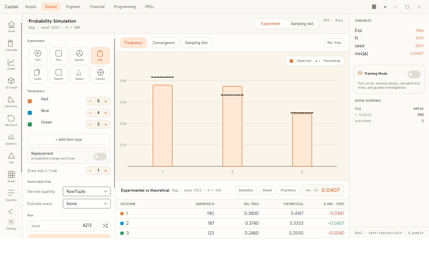
Reading the chart. Three tabs across the top of the workspace switch the view:

• Frequency draws a bar per outcome. Each solid bar is the observed relative frequency; a short dashed line across the top of each bar marks the theoretical probability. As trials accumulate the bars rise or fall to meet their dashes. A chip on the right toggles the y-axis between Rel. freq and raw Frequency.
• Convergence (below) traces the running relative frequency as one continuous line against the number of trials.
• Sampling dist. shows the dot/bell view used by the Central Limit demonstration.

Reading the table. The Experimental vs theoretical table under the chart lists one row per outcome with five columns: OUTCOME, OBSERVED N (the raw count), REL. FREQ (observed count over N), THEORETICAL (the exact probability), and Δ OBS − THEO (the signed gap, tinted so you can see at a glance which outcomes are running high or low). A max |Δ| readout beside the table header reports the single largest gap across all outcomes — the number to watch shrink as you add trials. A Fractions chip switches the relative-frequency column from decimals to stacked fractions.

The law of large numbers, on screen

The whole surface is built around one idea: the more trials you run, the closer the observed relative frequency sits to the true probability. This is the law of large numbers. A handful of trials can look lopsided — five coins might all come up heads — but as N climbs into the hundreds and thousands the wobble averages out and each observed frequency homes in on its theoretical value.

The Convergence tab makes this visible directly. It plots the running relative frequency of your chosen event as a single line while the number of trials grows along the horizontal axis. Early on the line swings widely; further right it flattens and hugs the dashed theoretical line. Small milestone chips along the top (10, 100, 1k) mark how far the line still sits from the target at those trial counts, and that gap steadily narrows.

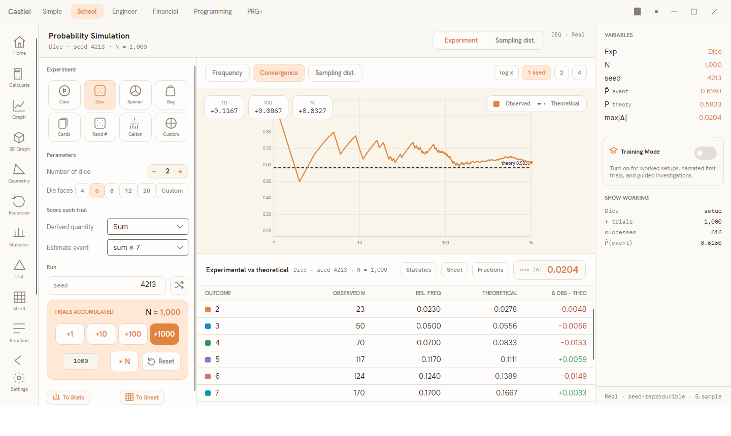
Two chips refine the view: an x-axis toggle switches the trial-count axis between log and linear (log spacing makes the early swings and the late settling both readable on one screen), and the 1 seed / 2 / 4 chips overlay several independent runs at once, so you can see that different random sequences all converge to the same line by different wobbling paths.

Worked example — a fair-looking biased spinner. The hero screenshot above runs the four-sector spinner with weights 5 : 3 : 3 : 1.

1. Select Spinner. In the bias editor set the four sector weights to 5, 3, 3, and 1; the probability bars read about 0.417, 0.250, 0.250, and 0.083, and the footer badge flips to biased.
2. Leave Derived quantity on RawTuple so each sector is tallied on its own, and Estimate event on None.
3. Press +100 a few times, or +1000 once. Watch the Frequency bars climb toward their dashed theoretical marks.

After 500 trials the table shows sector 1 at an observed 0.3920 against a theoretical 0.4167 (a gap of −0.0247), while sector 3 sits exactly on 0.2500. Keep adding trials and max |Δ| shrinks: the observed bars press ever closer to the dashed lines, and the wide first sector stays visibly the most likely — the point of the demonstration is that the biased wheel is genuinely biased, and the simulation reproduces that bias. Try it once more after pressing the shuffle button to change the seed; the individual counts differ but the same convergence holds.

The Galton board

The Galton experiment (also called a bean machine) drops balls through a triangle of pegs. At each of the Rows pegs a ball bounces left or right — a coin flip with probability P(right) — and lands in one of the bins at the bottom. Because each landing bin counts how many rights a ball took on the way down, the pile of balls builds the binomial shape: rare at the edges, tall in the middle.

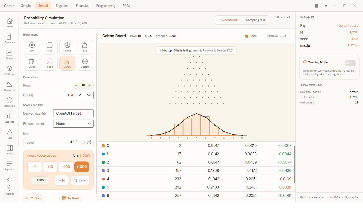
The board animates the balls falling, and the histogram of bin counts grows beneath it. A smooth binomial curve is overlaid (labelled Binomial(rows, p)) so you can compare the observed pile against the exact distribution, and the same comparison table lists each bin's observed count, relative frequency, theoretical probability, and gap. With P(right) at 0.50 the shape is symmetric; lower or raise it and the pile leans. The Galton board is the clearest picture of how many independent yes/no choices add up into a bell-shaped whole.

The sampling distribution (Central Limit Theorem)

Switch the top segment to Sampling dist. to run a different kind of demonstration. Here each sample is a batch of n trials, and the surface plots not the outcomes themselves but a statistic computed from each sample — either the sample Proportion or the sample Mean, chosen with the Measure chips. Every sample contributes one dot; together the dots build the sampling distribution of that statistic.

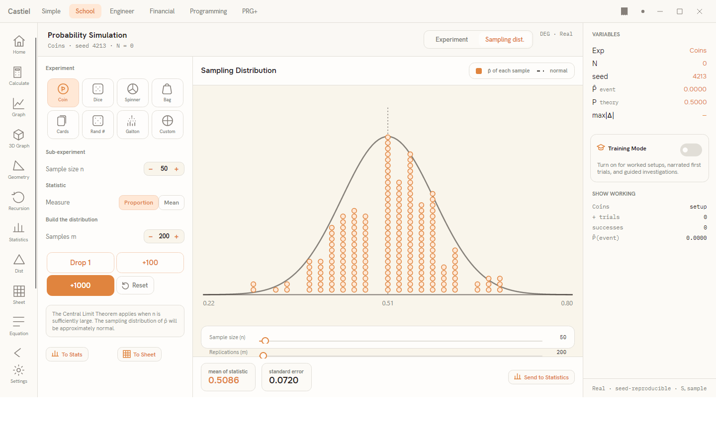
The setup column exposes three controls: Sample size n (how many trials go into each sample), the Measure, and Samples m (how many samples to build the distribution from). The action buttons Drop 1, +100, and +1000 add samples; Reset clears them; two sliders below the chart adjust n and m live. As samples accumulate the dots pile into a bell, and a smooth normal curve is drawn over them. Two readouts at the bottom report the mean of statistic and the standard error (how tightly the statistic clusters). This is the Central Limit Theorem in action: whatever the underlying experiment, the distribution of a sample statistic tends toward a normal curve as the sample size grows — and the note in the setup column says as much. Raising n with the slider visibly narrows the bell.

A Send to Statistics button hands the collected values to the Statistics app for further analysis; the experiment views offer the same routing through To Stats and To Sheet buttons.

Show working, aids, and Training Mode

The right side panel keeps a running account of what you did. Variables lists the live quantities — the experiment, the trial count N, the seed, the estimated probabilities, and max |Δ|. Show working logs the setup and each batch of trials into the shared paper tape, so the run becomes part of the same record every School surface writes to; see the paper tape for how that log is edited and exported.

Between them, context aids appear as small cards to head off common misconceptions (for instance, that a run of heads makes tails "due"). A Training Mode switch turns on worked setups, narrated first trials, and a numbered checklist of guided steps, with a Push working to tape button to record the guided run. Leave it off for free exploration; turn it on when you want the surface to walk you through an investigation.

Related chapters

• Distributions — the exact distribution curves the simulation converges toward.
• Statistics — summarise and chart the values you send across from a run.
• Probability distributions — the theory behind the binomial and normal shapes seen here.
• The School apps — Graph, Equation, Sheet, and the rest of the rail.
• The paper tape — where Show working records your run.