Chapters
The School inequality solver
The inequality solver is where you solve for a region of the number line rather than a single answer. Its sibling, the Equation app, finds the discrete values that make two sides equal; the inequality solver finds every value that makes one side larger or smaller than the other - and shows that answer three ways at once: shaded on a number line, written as intervals, and written as inequalities. You reach it from the Inequality tile on the left apps rail.
Use it whenever a problem asks "for which values of x is this true?": a linear inequality that solves to a single ray, a quadratic that opens into a union of two intervals, a rational expression with an excluded pole, an absolute-value band, or two conditions joined by and / or. It is a teaching surface as much as a solver - turn on Training Mode and it shows the sign chart and the reasoning behind every result.
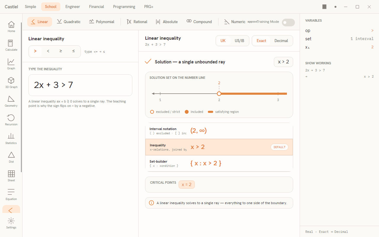
The window has three regions. Across the top is the mode bar - the row of inequality-type buttons - with the Training Mode switch at its right end. Below that the workspace splits in two: a narrow entry spine on the left where you type the inequality and pick the relation, and the wide result panel (the solution readout) on the right. A third Variables / Show working panel runs down the far-right edge, mirroring the result into the shared paper tape.
The seven inequality types
The mode bar groups the types into three tiers, separated by thin dividers. Pick a type and the entry spine and result panel switch to match it.
| Type | What it solves | Example you start from |
|---|---|---|
Linear |
ax + b ⋛ 0 - solves to a single ray |
2x + 3 > 7 |
Quadratic |
ax² + bx + c ⋛ 0 - an interior interval or an outside union |
x² − 5x + 6 > 0 |
Polynomial |
higher-degree p(x) ⋛ 0, driven by a sign chart |
x³ − 6x² + 11x − 6 < 0 |
Rational |
a quotient p(x)/q(x) ⋛ 0, with excluded poles |
(x − 1)/(x + 2) ≥ 0 |
Absolute |
|f| ⋛ k - a bounded band or an outside union |
|2x − 1| > 3 |
Compound |
two conditions joined by and / or | 1 < x and x ≤ 5 |
Numeric |
an arbitrary f(x) ⋛ g(x) solved by scanning a window |
e^x > 2x + 2 |
The first three (Linear, Quadratic, Polynomial) are the core tier. Rational, Absolute, and Compound are the next tier. Numeric stands alone as an optional tier and carries a small approx label, because it works by sampling rather than by exact algebra - its answers are always marked approximate (see Special cases and approximate results).
Every type opens seeded with a worked demo, so the surface is never blank. Clear the entry and type your own.
Entering an inequality
Typing the expression. For every type except Compound, the entry spine gives you one box headed TYPE THE INEQUALITY (or TYPE THE QUOTIENT INEQUALITY / TYPE THE ABSOLUTE-VALUE INEQUALITY for those modes). Write the inequality the way it reads on paper, including the relation: x² − 5x + 6 > 0. The solution updates as you type. A short note under the box explains the teaching point of the active type.
Choosing the relation. Above the entry box sits the operator chooser, a four-button toggle: >, <, ≥, ≤. It mirrors whatever relation you typed, and pressing one of its buttons rewrites the relation in the entry to match - so the toggle and the typed text always agree. You can type the plain forms <= and >=; they are shown as ≤ and ≥, and a hint beside the chooser (type <= → ≤) reminds you of this. The operator chooser is hidden in Compound mode, because there each condition carries its own relation.
Compound conditions. Compound mode replaces the single box with two - CONDITION 1 and CONDITION 2 - and a JOIN control between them offering AND and OR. AND keeps only the overlap of the two conditions (their intersection); OR keeps everything in either (their union). You can also write a chained condition directly in one box, such as 1 < x ≤ 5.
Numeric scanning. Numeric mode adds a SCAN WINDOW with a low and a high bound and a Scan button. It compiles your f(x) and g(x), then sweeps a fine grid across the window looking for where the relation holds. Results outside the window are not covered, and a boundary where the two curves only just touch can be missed - which is why this mode is always approximate.
Reading the solution
The result panel presents the same solution set several complementary ways. From the top:
The headline states the shape of the answer in words - "Solution - a union of 2 intervals", "Solution - a single unbounded ray", or one of the special outcomes below - with a check mark beside it and, to its right, an op-applied chip restating the answer in inequality form (for example x < 2 or x > 3).
The number line is the centrepiece, labelled SOLUTION SET ON THE NUMBER LINE. The satisfying region is drawn as a shaded bar; the critical points are marked and labelled; and the endpoints tell you whether each boundary is included. Its legend spells out the three marks:
- an open circle - the endpoint is excluded (a strict
<or>, or an excluded pole); - a filled dot - the endpoint is included (an inclusive
≤or≥); - a shaded bar - the satisfying region itself.
This open-versus-closed distinction is the whole grammar of the diagram: x > 3 draws an open circle at 3 with the bar running right; x ≥ 3 draws a filled dot. A Rational pole is always drawn as a red open hole, excluded even when the relation is ≥ or ≤, because the expression is undefined there.
The triple notation shows the answer as three rows at once, so you can read whichever your course expects:
| Row | Reads the solution as | Example |
|---|---|---|
| Interval notation | brackets - ( ) excludes an endpoint, [ ] includes it |
(−∞, 2) ∪ (3, ∞) |
| Inequality | x-relations joined by or / and |
x < 2 or x > 3 |
| Set-builder | { x : condition } |
{ x : x < 2 or x > 3 } |
One row is flagged DEFAULT. Which one depends on the notation-region toggle in the result-panel header: UK makes the inequality row the default, US/IB makes interval notation the default. The toggle only changes which row is highlighted - all three are always shown.
The critical points appear as a compact strip of chips (x = 2, x = 3, …); a pole chip is tinted red to distinguish it from an ordinary root.
Interval notation versus inequality notation
The two notations describe the same set with opposite emphasis, and the number line ties them together. Take the linear demo 2x + 3 > 7, which solves to x > 2:
- Inequality notation names the variable and its relation to the boundary:
x > 2. It is the natural reading of the number line - "everything to the right of 2, boundary open." - Interval notation names the span of values with brackets:
(2, ∞). The round bracket at 2 means 2 is excluded (matching the open circle); a square bracket would mean it is included. Infinity always takes a round bracket, because there is no endpoint to include.
For a union of intervals the two stay in step. A quadratic that is positive outside its roots reads x < 2 or x > 3 as inequalities and (−∞, 2) ∪ (3, ∞) as intervals - the ∪ (union) symbol joining the two spans is the same "or" written another way.
Special cases and approximate results
Not every inequality solves to a tidy interval. The result panel calls out the special outcomes with a banner:
- No solution (
∅). No real number satisfies the inequality - the empty set. This is what|f| < a negative numbergives, or a quadratic whose parabola never reaches the far side of the relation. - All real numbers (
ℝ). Every value works, and the whole line is shaded. This is|f| > a negative number, or a quadratic with no real roots sitting entirely on the satisfying side. - All reals except one point (
ℝ∖). The whole line minus a single open hole, such as the solution of(x − 2)² > 0, which is every value exceptx = 2. - Exactly one solution (
•). A single filled dot where the expression is zero and nowhere else.
For a quadratic, the discriminant b² − 4ac is what decides between these: a negative discriminant means no real roots, so the parabola keeps one sign and the answer is all-reals or empty - never a complex root. Training Mode states the discriminant and its consequence as a caption.
Approximate answers. Two situations produce boundaries that cannot be found exactly: a polynomial above degree 4 (no general exact factoring exists) and any Numeric scan. In both, the result panel shows a Numerical boundaries · approximate badge so you know the endpoints are computed values, not exact ones.
Exact versus decimal endpoints
The result-panel header carries an Exact / Decimal toggle, and the solver prefers exact. Where a boundary is a rational number it is shown as an exact fraction - 3/2 rather than 1.5 - in every notation at once. Switch to Decimal and the same boundaries re-render as rounded decimals, without re-solving. An irrational boundary (such as a surd root) has no exact fraction, so it is shown as a decimal even in Exact mode. The toggle changes only how the numbers are written; the solution set is unchanged.
Training Mode and the sign chart
The Training Mode switch at the top right turns the solver from an answer engine into a worked lesson. With it on:
- each type shows its teaching caption under the result - why the sign flips when you divide a linear inequality by a negative, why you must not multiply a rational inequality across its denominator, how a case split turns
|f| > kinto an outside union, and so on; - the sign chart appears. This is the table headed
SIGN CHART: the critical points split the line into columns, thef(x)row shows the sign of the expression (+,−, or0) in each column, and the columns that satisfy the inequality are highlighted. Its note reminds you to test a point in each interval, and that an even-multiplicity root only touches the axis (no sign change) while an odd one crosses; - a Push working button appears on the right panel, writing the full derivation - coefficients, discriminant, critical points, the relation applied - into the Show working list.
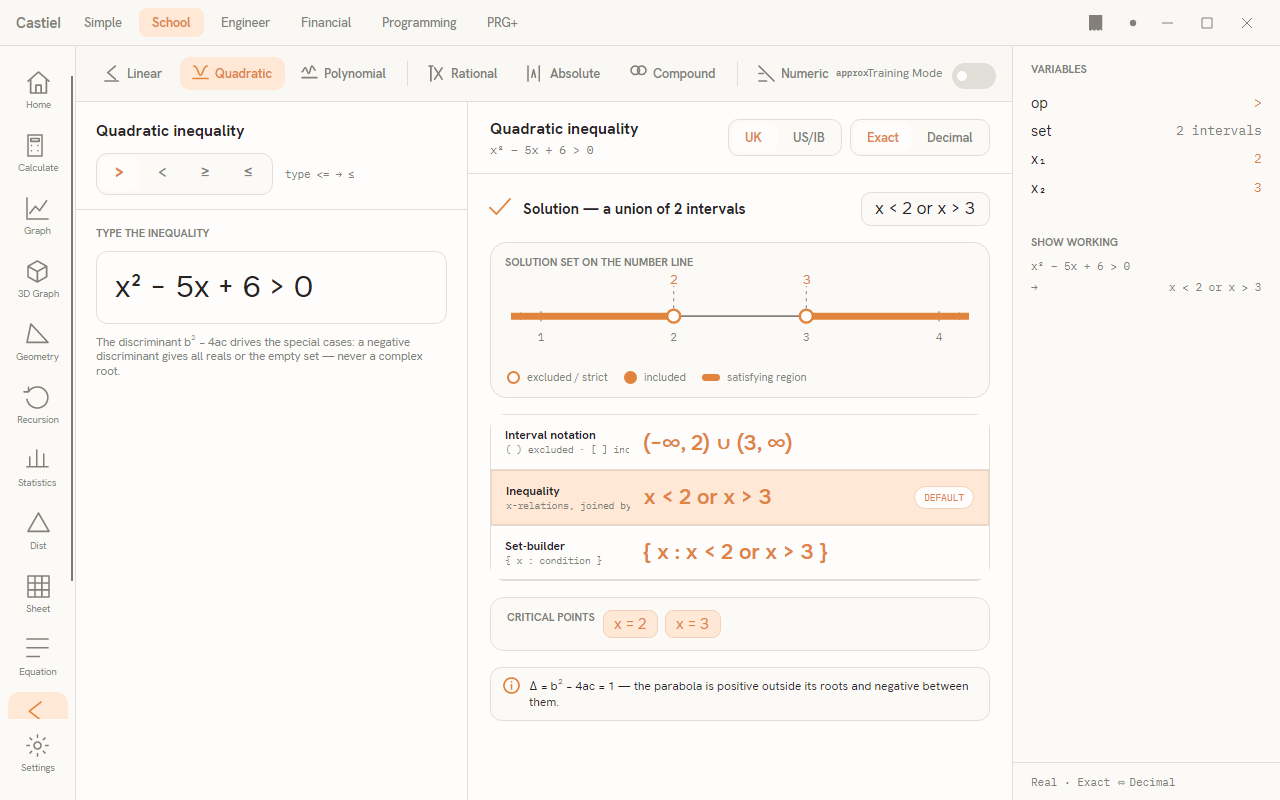
A worked example: a quadratic union
Solve x² − 5x + 6 > 0 and read off the union of intervals.
- Choose the
Quadratictype on the mode bar. - In the entry box type
x² − 5x + 6 > 0. The operator chooser lands on>to match. - Read the result. The expression factors as
(x − 2)(x − 3), so the critical points arex = 2andx = 3- shown as two chips and two labelled marks on the number line. Because the parabola opens upward, it is positive outside its roots, so the satisfying region is the two outer rays.
The answer appears in all three notations at once:
- Inequality:
x < 2 or x > 3 - Interval:
(−∞, 2) ∪ (3, ∞) - Set-builder:
{ x : x < 2 or x > 3 }
Both endpoints are open circles, because the relation is strict (>): 2 and 3 are the boundaries but are not themselves solutions. Switch the relation to ≥ and the two circles fill in and the notation brackets close to (−∞, 2] ∪ [3, ∞). Turn on Training Mode to see the sign chart confirm it: + on the outer columns (highlighted), − between the roots.
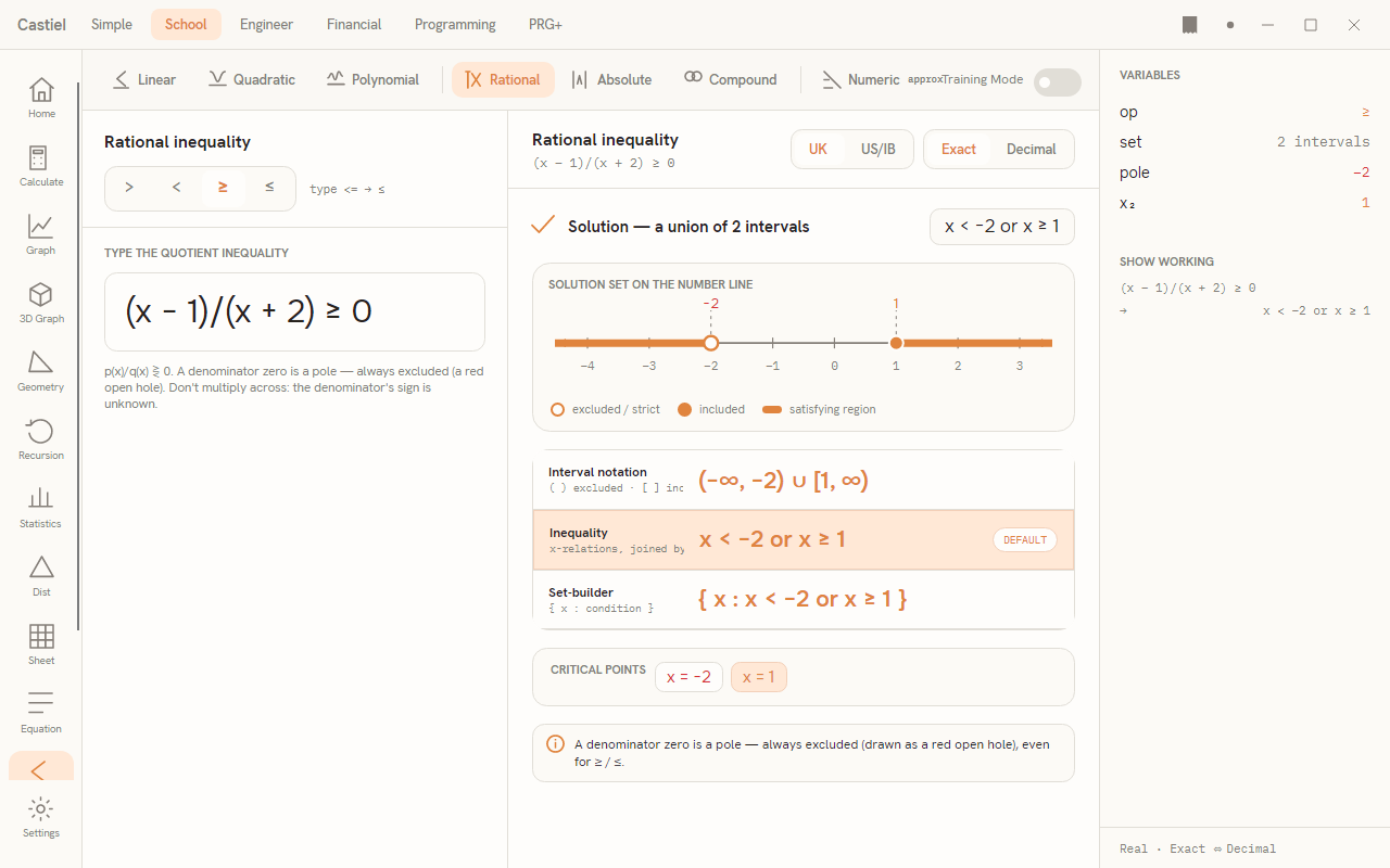
The Rational type is worth contrasting here. Solving (x − 1)/(x + 2) ≥ 0 gives a root at x = 1 (a filled dot, since ≥ includes it) but a pole at x = −2 - where the denominator is zero and the expression undefined. The pole is drawn as a red open hole and is always excluded, even though the relation is inclusive.
Compound conditions and the paper tape
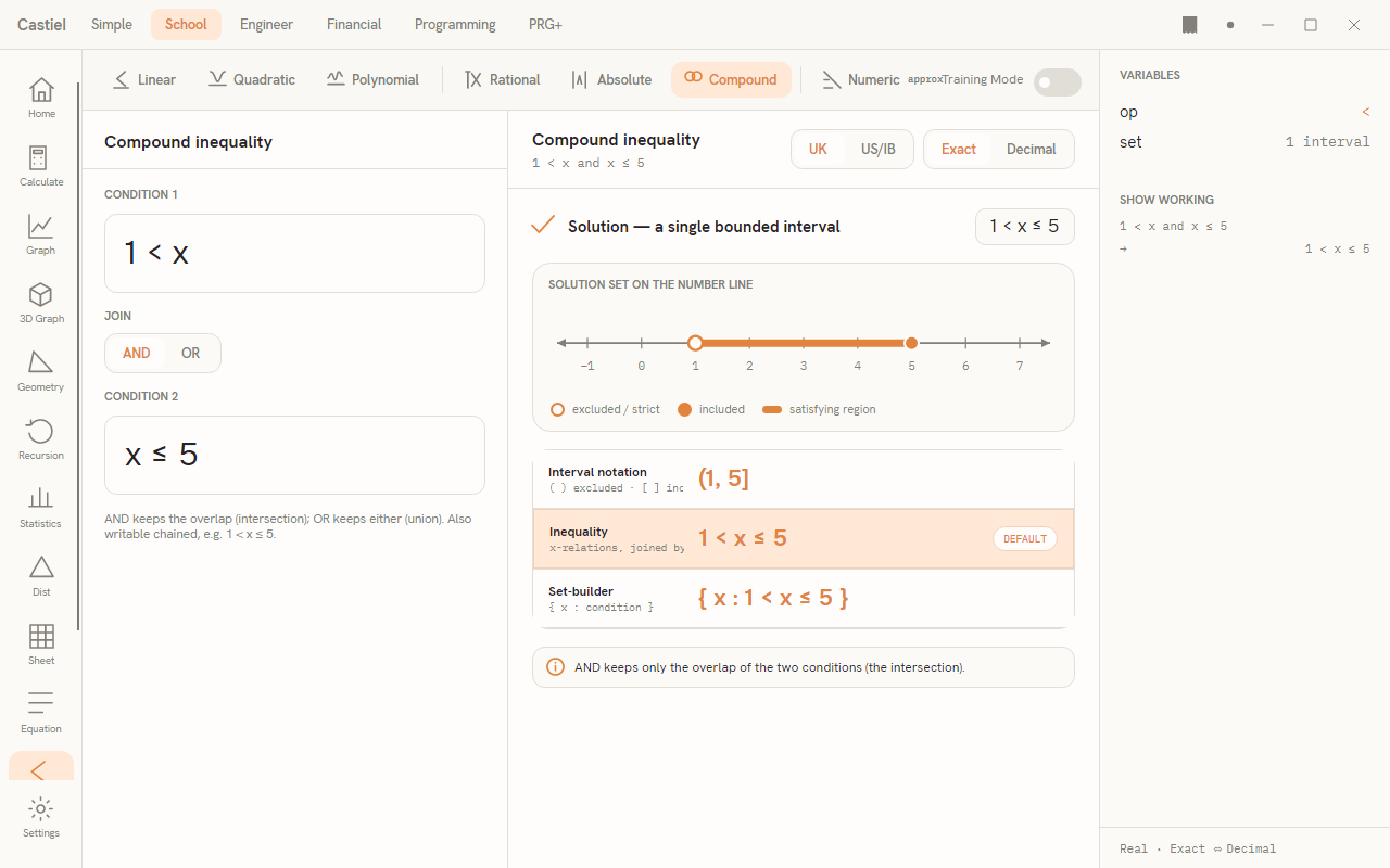
Compound mode joins two conditions and shows the result of the join. 1 < x and x ≤ 5 keeps only the overlap - 1 < x ≤ 5, the interval (1, 5] with an open left endpoint and a closed right one. Switch the join to OR and the answer keeps everything in either condition; where the two conditions leave a gap, that gap is the region in neither, and the number line shows it unshaded.
The far-right panel is the surface's link to the shared paper tape. Its Variables list carries the relation, the shape of the solution (how many intervals, or ∅ / ℝ), and the critical points and poles. Below it, Show working holds a compact tape line for the current solution; pressing Push working in Training Mode replaces it with the full derivation. This is the same tape that runs through every School app - see the paper tape for editing and exporting it.
Related chapters
- The School equation solver - its sibling, for solving for exact roots rather than a region.
- The School graph - plot the same expression to see the inequality's regions as areas of the curve.
- The School apps - Calculate, Graph, Equation, and the rest of the rail.
- The paper tape - editing, correcting, and exporting your working.