Chapters
The School equation solver
The Equation solver is the School app for finding the values that make an equation true. You reach it from the Equation tile on the left apps rail. Where the School calculator evaluates one expression, this surface solves - it takes a system of equations, or a single polynomial, and returns the unknowns. It gathers four related solvers under one roof: a Linear systems solver for simultaneous equations, a Quadratic solver, a general Polynomial solver by degree, and a Numeric solver that finds roots of any equation you can type.
Use it whenever the question is "what is x?" rather than "what is this expression worth?" - solving two equations in two unknowns, applying the quadratic formula, factoring a cubic, or pinning down a root of something like sin(x) = x/3 that has no neat closed form. For a single evaluation, use Calculate; for inequalities, see the sibling Inequality solver.
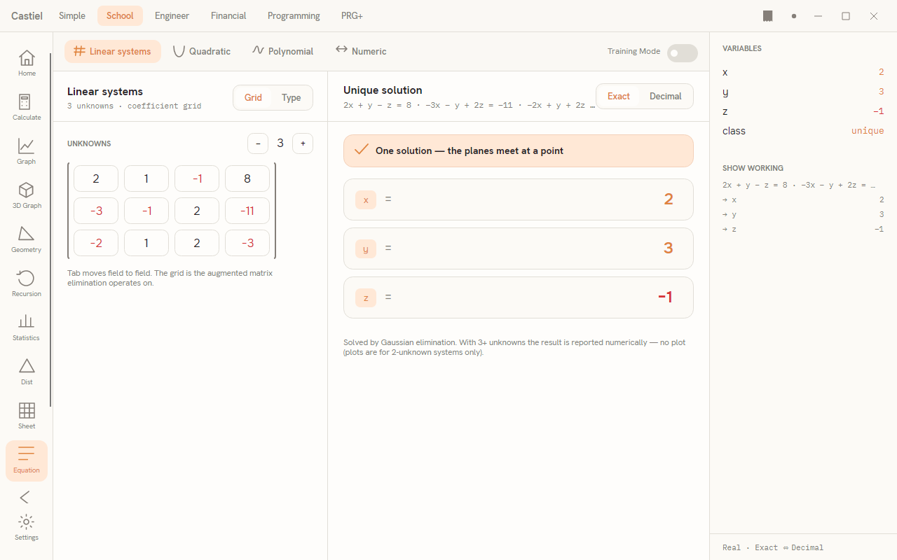
The window has three regions. Across the top is the solver strip: the four solver tabs (Linear systems, Quadratic, Polynomial, Numeric) on the left, and a Training Mode switch on the right. Below that, the workspace splits in two: an entry spine on the left where you type coefficients or an equation, and a result panel on the right that shows the solution, a plot, and any special-case explanation. Down the far right is the Variables / Show working panel, a live readout of the solved unknowns and a compact record of each solve.
Every solver opens with a worked example already in place, so you can see the shape of a solution before typing your own.
The controls every solver shares
Switching solvers. Click a tab in the top strip. The entry spine and result panel both change to match, and the surface re-solves whatever example is loaded so the panel is never blank.
Exact versus decimal. The result panel header carries an Exact / Decimal toggle. Exact is the default: where a solution can be written as a whole number, a fraction, or an exact form, that is what shows. Decimal switches every figure in the panel to its decimal value. The toggle only changes how the numbers are displayed - it never re-solves and never changes the value. (The Numeric solver is the exception: its roots are decimal by nature, so the toggle leaves them unchanged.)
Training Mode. The switch at the top right turns on the teaching view. With it off, each solver gives you the answer and a plot. With it on, the result panel also shows the worked steps - the elimination for a linear system, the quadratic-formula derivation, or the iteration trace for the Numeric solver - and a Push working button appears above the right panel that copies the full derivation into the Show working list.
The right panel. VARIABLES lists the solved unknowns and a little classification metadata (for a linear system, its class; for a quadratic, the discriminant Δ). SHOW WORKING keeps a compact line-by-line record of the current solve. The foot of the panel reads Real · Exact ⇔ Decimal, a reminder of the current number domain and display mode.
Linear systems
The Linear systems solver handles simultaneous linear equations in 2 to 6 unknowns. Set the number of unknowns with the − / + stepper labelled UNKNOWNS; the entry area reshapes to match, and the unknowns are named x, y, z, u, v, w in order.
Two ways to enter the system. The Grid / Type segmented control at the top of the entry spine chooses between them:
- Grid gives you an editable coefficient grid - the augmented matrix. Each row is one equation; the columns are the coefficients of each unknown, and the last, set-off column is the constant on the right-hand side. Tab moves from cell to cell. In the screenshot above, the first row
2 1 −1 8stands for2x + y − z = 8. - Type lets you write one equation per line in natural form, such as
2x + 3y = 7. As you type, a Parsed confirmation shows the same system as a matrix so you can check the translation before trusting it.
Either way the system re-solves as you edit.
Reading the result. Every linear result is classified into one of three cases, each with its own coloured verdict banner:
| Case | Verdict | What it means |
|---|---|---|
| Unique solution | One solution - the lines (or planes) meet at a point | Exactly one set of values satisfies every equation; each unknown gets its own result row. |
| No solution | Inconsistent - no solution | The equations contradict each other. For two unknowns, the lines are parallel and never meet: the coefficients are proportional but the constants are not. |
| Infinitely many solutions | Dependent - infinitely many solutions | The equations describe the same line, so every point on it works. The panel prints a general solution in a free parameter t ∈ ℝ, for example x = 2 − t, y = t. |
For a two-unknown system the panel also draws the two lines so you can see the geometry - they cross at the solution, run parallel when there is none, or lie on top of each other when there are infinitely many. With three or more unknowns there is no plot; the panel notes that plots are for two-unknown systems only and reports the result numerically.
Training Mode adds the full Gaussian elimination - each row operation (swap, normalise, eliminate) shown as a numbered step with the matrix after it - followed by a back-substitution check that puts the solution back into each original equation to confirm LHS = RHS, and a hint about the common trap of confusing a dependent system with an inconsistent one.
Worked example - a two-unknown system. The solver opens on the system
2x + 3y = 7
4x − y = 1- Leave the entry on
Type(or switch toGridand read off the coefficients). - The result panel shows the green Unique solution verdict and two rows:
x = 5/7andy = 13/7, stacked as exact fractions. - Press
Decimalon the header toggle to read them as0.714…and1.857…; pressExactto return to the fractions. - Below, the two lines are plotted crossing at the single point
(5/7, 13/7).
Quadratic
The Quadratic solver works on ax² + bx + c = 0. Type the equation in natural form in the TYPE THE EQUATION box (the default is x² − 5x + 6 = 0), or switch the Grid / Type control to Grid and fill the a, b, c coefficient cells directly. If you leave a at zero the panel reminds you that a must be non-zero for a quadratic.
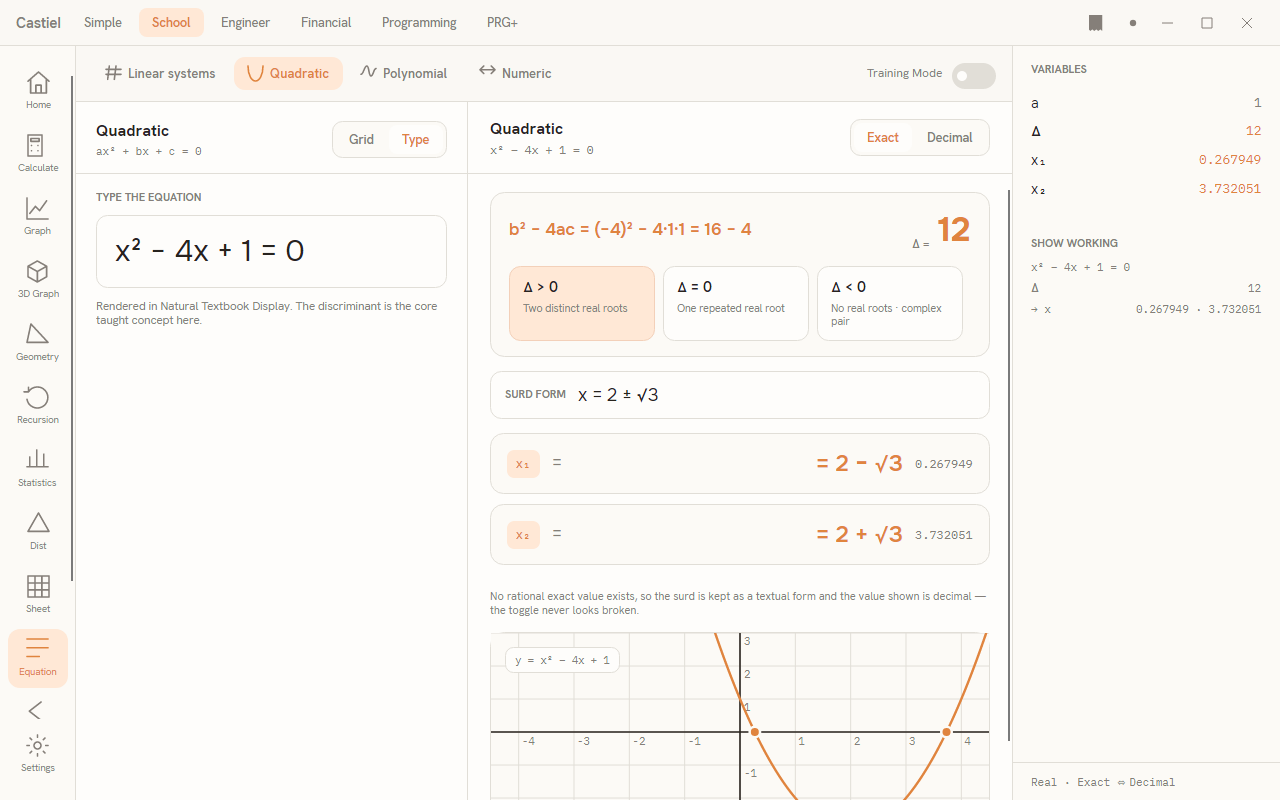
The discriminant card. The heart of this solver is the discriminant, b² − 4ac, written out with your numbers substituted in (for x² − 4x + 1 it reads (−4)² − 4·1·1 = 16 − 4) and its value Δ shown to the side. Three chips beneath it - Δ > 0, Δ = 0, Δ < 0 - light up the one that applies, because the sign of the discriminant decides the character of the roots:
Δ > 0- two distinct real roots.Δ = 0- one repeated real root.Δ < 0- no real roots; a complex conjugate pair instead.
Reading the roots. When the roots are rational they appear as exact values (whole numbers or fractions) that you can toggle to decimal. When they are irrational, the panel shows the surd form as a caption - for example x = 2 ± √3 - with each root row carrying the surd beside its decimal value.
There is an important subtlety here. Castiel does not carry irrational roots as a re-computable exact type. The surd 2 ± √3 you see is a rendered text label that describes the value; the number the solver actually holds and reuses is the decimal (0.267949…, 3.732051…). The panel says as much: no rational exact value exists, so the surd is kept as textual form and the figure shown stays decimal - which is why the Exact / Decimal toggle does not "break" on a surd, it simply has no separate exact number to switch to. Read the surd as the exact description, and the decimal as the value you compute with.
Complex roots. When Δ < 0 the panel leads with a plain "No real solutions" note - the parabola never crosses the x-axis - and then presents the roots as a conjugate pair a ± bi in a clearly marked further-study block. Complex roots are always shown, never suppressed; they simply come after the school-level explanation.
Every quadratic also gets its parabola plotted, with the real roots marked where the curve meets the axis. Training Mode adds the step-by-step derivation - identifying the coefficients, forming the discriminant, and applying x = (−b ± √(b² − 4ac)) / 2a - plus a hint watching the sign of −b and the easily dropped ±.
Worked example - an irrational quadratic. Enter x² − 4x + 1 = 0:
- The discriminant card reads
(−4)² − 4·1·1 = 16 − 4, withΔ = 12. TheΔ > 0chip lights, so expect two distinct real roots. - Because 12 is not a perfect square, the roots are irrational: the surd form caption shows
x = 2 ± √3. - The two root rows read
x₁ = 2 − √3with decimal0.267949, andx₂ = 2 + √3with decimal3.732051. - Pressing
Decimalleaves those figures as they are - the surd is the exact description, the decimal is the value.
Polynomial
The Polynomial solver takes a single-variable polynomial equation of degree 2 to 6, typed in natural form (the default is x³ − 6x² + 11x − 6 = 0). A DEG badge in the entry header echoes the degree it read.
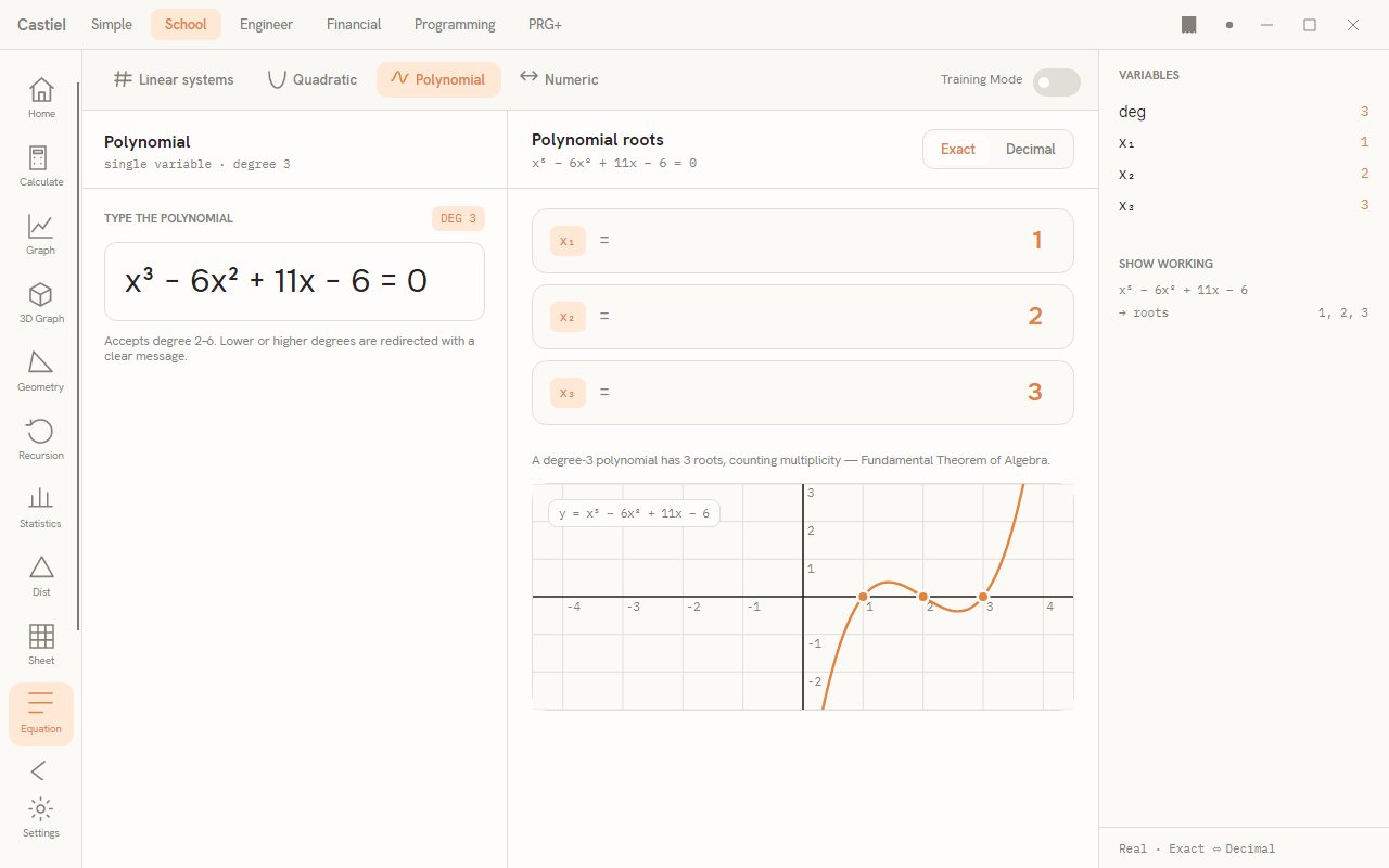
It returns all the roots. Real roots are listed first, exact where they are rational; a repeated root carries a multiplicity badge (for instance multiplicity 2). Complex roots follow in a labelled conjugate-pair block and, like everywhere else, are never hidden. A caption states the count as the Fundamental Theorem of Algebra guarantees it: a degree-n polynomial has n roots, counting multiplicity. The curve y = f(x) is plotted with the real roots marked.
If you type something outside degree 2–6 - a linear expression, or a degree-7-and-up polynomial - the solver does not fail silently. It explains that this surface covers degree 2 to 6 and offers an Open in Numeric solver button that carries your equation straight over to the Numeric tab, which can find roots in a range for any degree.
For the example above, x³ − 6x² + 11x − 6 = 0 resolves to three distinct real roots, x₁ = 1, x₂ = 2, x₃ = 3, and the cubic is drawn crossing the axis at each.
Numeric
The Numeric solver finds roots of an equation that need not be polynomial at all. Type it as f(x) = g(x) (the default is sin(x) = x/3) and the solver works on f(x) − g(x) = 0 - that is, it hunts for the x where the two sides are equal. Everything here is decimal: transcendental roots have no exact form.
The FIND ROOTS BY control chooses the method:
- Auto-scan samples a range you set with the low and high boxes and press Scan range on. It returns every root where the function changes sign across that interval, not just one - useful when an equation has several roots and you want them all. If no sign change is found, the panel suggests widening the range or warns that there may be no real root in that interval.
- Manual guess takes a single starting value
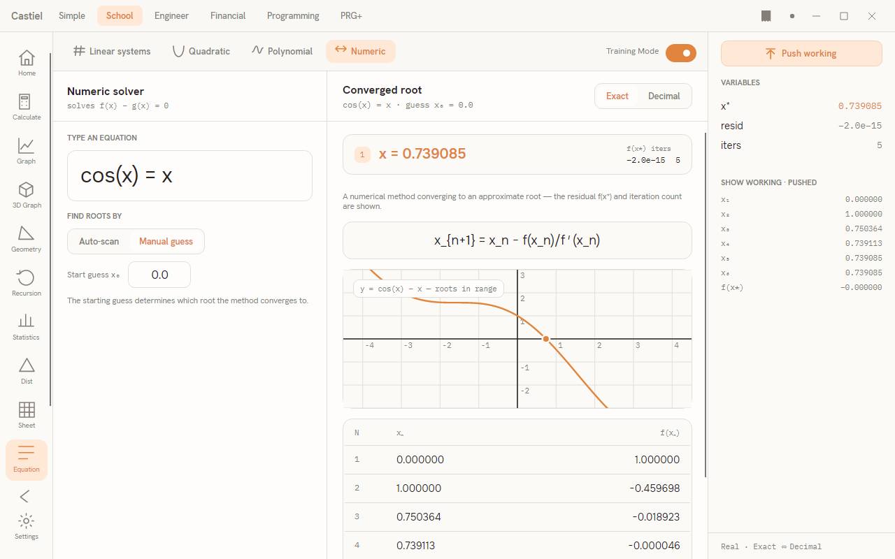
x₀and refines it with Newton's method, following the tangent downhill to the nearest root. The starting guess decides which root you land on when there are several.
Each root is reported with its value x, the residual f(x*) (how close to zero the function actually is there - a measure of accuracy), and the iteration count it took to get there.
When Newton's method does not converge. Newton's method can stall - most often near a turning point, where the slope f′(x) is close to zero, the tangent is nearly flat, and the next step shoots far away. Rather than spin or return nonsense, the solver stops and gives plain-language guidance: it tells you the method stalled at a turning point, and suggests trying a different starting guess or switching to Auto-scan, while noting the equation may simply have no real root there.
Training Mode (with Manual guess) reveals how Newton's method reached the answer: the update formula xₙ₊₁ = xₙ − f(xₙ)/f′(xₙ), and a trace table listing each iteration N, the running estimate xₙ, and the value f(xₙ) - which you can watch shrink toward zero row by row. In the screenshot, cos(x) = x is solved from x₀ = 0, converging to x = 0.739085 after five iterations, with the residual collapsing to essentially zero.
Results and the Show working panel
The right-hand Variables / Show working panel is this surface's running record. After each solve, VARIABLES holds the solved unknowns and their classification, and SHOW WORKING keeps a compact summary line - the equation you solved and the values it produced.
In Training Mode, the Push working button (above the panel) copies the full derivation into SHOW WORKING - the elimination rows for a linear system, the discriminant and formula for a quadratic, or the whole Newton trace for a numeric solve - and the header changes to SHOW WORKING · PUSHED to mark that the detailed version is now captured. This is how you turn a solve into a written record you can review step by step, the same way the paper tape keeps your work in the other School apps.
Related chapters
- The School calculator - evaluating single expressions, and the Natural Textbook entry used across School.
- Inequality - solving inequalities rather than equations.
- Numerical methods - root-finding, Newton's method, and iteration in depth.
- The School apps - Graph, Statistics, Equation, and the rest of the rail.