Chapters
The Engineer plot
The Engineer Plot surface is Castiel's function grapher for advanced work. You reach it from the Plot tile on the Engineer sub-app rail down the left edge (Calculate, CAS, Matrix, Vector, Units, Const, Plot, Numeric, Settings). Where the School Graph is built for everyday y = f(x) curves, the Engineer Plot adds two more coordinate systems - polar and parametric - alongside the Cartesian one, and it carries a compact analysis toolbar for tracing curves, zooming the view, and solving for roots and intersections.
Use it whenever you are working in Engineer mode and want to see a function rather than just evaluate it: to check the shape of a curve, find where two functions cross, locate a root, or draw a polar rose or a parametric path. For a step-by-step table of values, or for School-mode plotting, the School Graph is the better surface; for solving equations without a picture, see Numerical methods.
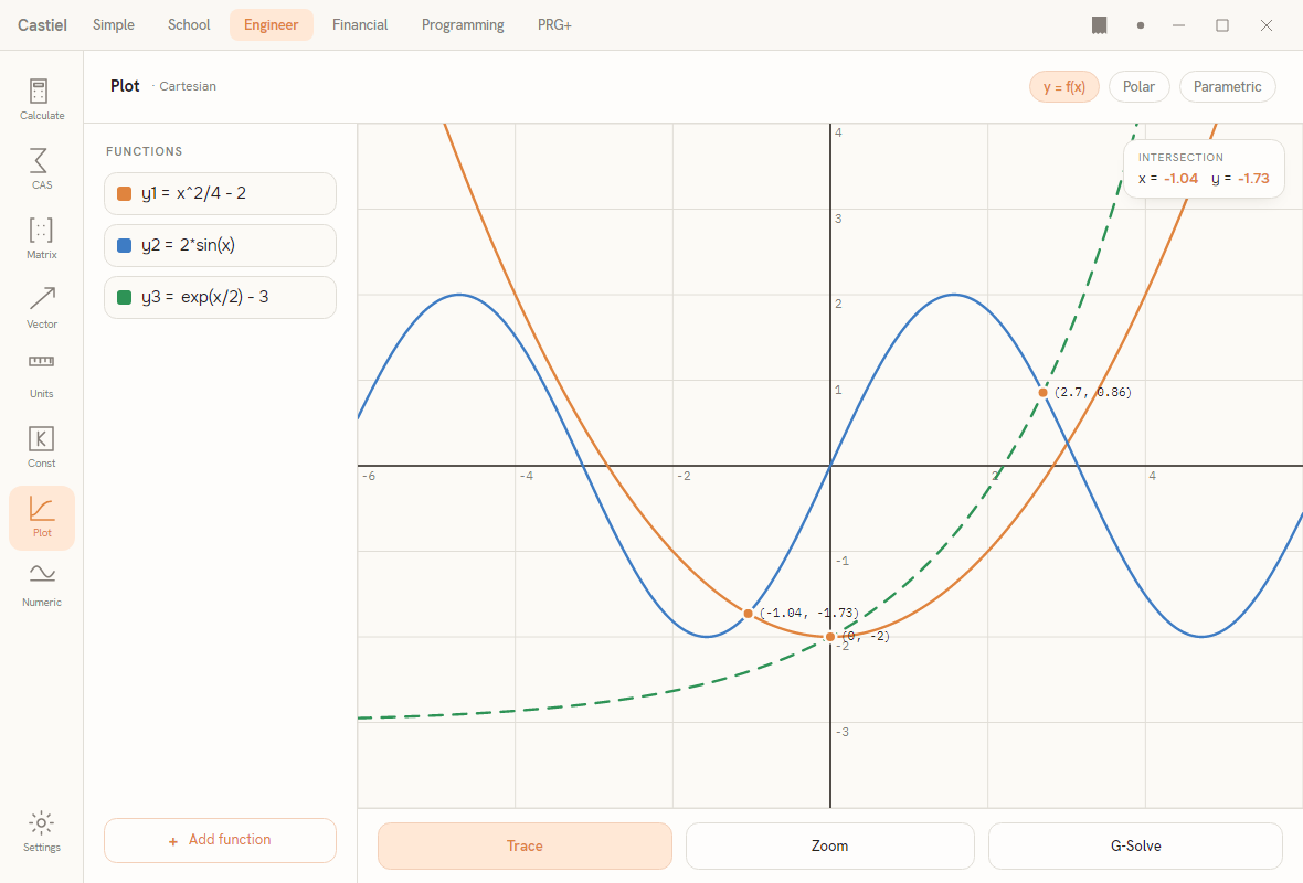
The surface has three parts: a header across the top with the surface title and the three plot-type pills; a function panel down the left (the colour-keyed list of curves plus an Add function button); and the plot canvas filling the rest of the window, with an analysis toolbar - Trace, Zoom, G-Solve - pinned along the bottom.
Choosing a plot type
The header reads Plot followed by the active plot type - Plot · Cartesian in the screenshot. Three pills on the right of the header switch between the coordinate systems:
| Pill | Plot type | What each curve is |
|---|---|---|
y = f(x) |
Cartesian | An ordinary function of x. Each row holds one expression in x, drawn as a height above the x-axis. |
Polar |
Polar | A radius as a function of the angle, r(θ). Each row holds one expression in theta, swept over an angle range. |
Parametric |
Parametric | A path traced by a point, given as a pair x(t) and y(t). Each row holds two expressions in t. |
Each plot type keeps its own separate function list. Switching type swaps the panel to that type's curves - nothing you typed is lost, and switching back brings your earlier list straight back. The view window is also preserved across a switch: the region of the plane you framed stays put when you flip between Cartesian, polar, and parametric, so you can compare the same patch of the plane in different coordinate systems.
Entering functions
The left Functions panel is the editable list of curves for the active plot type. Each row carries three things: a small colour swatch, a label, and an expression box you type into.
- The swatch colour is the colour that curve is drawn in on the canvas, so the list and the graph always match. In the screenshot,
y1is orange,y2is blue, andy3is green. - The label names the curve:
y1,y2,y3, and so on in Cartesian mode. Polar curves are labelledr, and parametric curves are labelled as a(x, y)pair. - The expression box is where you type the formula. Type it in ordinary linear form -
x^2/4 - 2,2*sin(x),exp(x/2) - 3- using^for powers,*for multiplication, and the function names from the engine (sin,cos,exp,ln, and the rest). The curve redraws as you type.
Add function at the foot of the panel appends a fresh empty row, so you can plot as many curves at once as you need. To change a curve, edit its box; to blank one out, clear its box.
A note on the variable name. The variable follows the plot type: use x in Cartesian expressions, theta in polar expressions, and t in parametric expressions. Writing the bare constant e is read as a variable, not Euler's number - spell the exponential as exp(...) when you mean eˣ (the seeded exp(x/2) - 3 curve is written this way for exactly that reason).
Parametric rows show two boxes instead of one: an upper box for x(t) and a lower box for y(t). A parametric curve needs both halves - fill in only one and the row is flagged as incomplete rather than drawn as half a curve.
The sweep range (polar and parametric). In Polar and Parametric types a range row appears at the foot of the panel, labelled θ range or t range. It sets the interval the parameter runs over - a from box, an arrow, and a to box. The default is one full turn (0 to about 6.283, i.e. 2π). Widen or narrow it to draw more or less of a polar rose or a parametric path. The range does not apply in Cartesian mode, where the curve simply spans the visible width of the canvas.
Reading and moving the view
The canvas draws the curves over a labelled grid with the axes through the origin. The Engineer default framing shows x from about -6 to 6 and y from about -4 to 4; the numbers along the axes tell you the scale at a glance.
The analysis toolbar along the bottom has three tools. Selecting one highlights it in the accent tint (in the screenshot Trace is active):
Tracewalks a point along a curve. As you trace, a readout card appears at the top-right corner of the canvas showing the curve you are on and the point's real coordinates - for exampleTRACE · Y1withx =andy =filled in. The coordinates are genuine evaluations of the function, not pixel estimates.Zoomlets you zoom the view in or out to reframe the plot. Because the framing is preserved across plot-type switches, a view you zoom to in Cartesian mode is the same view you return to in polar or parametric mode.G-Solveopens the analysis panel described below.
The readout card. Whether it is showing a trace, a root, or an intersection, the card follows the same shape: a small label naming what it holds (TRACE · Y1, ROOT · Y1, INTERSECTION, or CLOSEST APPROACH), then x = and y = values, and - for a closest approach - an extra Δ = line giving the separation between the two curves. Card values are shown to two decimals; the fuller precision appears in the G-Solve status line.
G-Solve: roots and intersections
Selecting G-Solve opens a small panel at the top-left of the canvas with three actions and a status line:
| Action | What it does |
|---|---|
Intersection |
Finds where curves cross. In Cartesian mode this is a true intersection: for every pair of curves the visible x-range is scanned and each pair's first crossing in view is marked. The card shows the first one found and the status line reports how many were found (2 intersections in view.). |
Root |
Cartesian only. Finds the first place the first curve crosses the x-axis inside the current view, and marks it. In polar or parametric mode the status line reminds you to use Intersection instead. |
Clear markers |
Removes the markers G-Solve has placed and clears the status line. |
Each solved point is marked on the canvas with its coordinates, and the readout card carries the headline result. Intersection needs at least two curves present; Root needs at least one.
Polar and parametric intersections. Two swept curves cross where different parameter values land on the same point of the plane - a harder question than a Cartesian crossing. Here Intersection reports the closest approach between the curves: if the two come together to essentially zero separation, the card says INTERSECTION; otherwise it says CLOSEST APPROACH and the Δ = line gives how near they came. This lets you find true crossings and near-misses of polar and parametric curves with the same button.
A worked example: where two curves meet
The screenshot has three Cartesian curves loaded: y1 = x^2/4 - 2 (a parabola), y2 = 2*sin(x) (a wave), and y3 = exp(x/2) - 3 (a rising exponential). To find where the parabola and the wave cross:
- Confirm the header shows
Plot · Cartesian(they = f(x)pill is on). - Check the two expressions are entered:
x^2/4 - 2iny1and2*sin(x)iny2. - Press
G-Solveon the bottom toolbar. - In the panel that opens, press
Intersection.
Castiel scans the visible x-range and marks each crossing. The readout card at the top-right reports the first one - INTERSECTION, x = -1.04, y = -1.73 - and the status line summarises the total found in view. The markers stay on the canvas so you can read every crossing at once; press Clear markers to remove them.
To find where the parabola alone meets the x-axis instead, leave y1 as the first curve, press G-Solve, then Root: the first in-view root is marked and the card reads ROOT · Y1.
How it differs from the School Graph
The two graphers share the same canvas, the same trace and zoom behaviour, and the same colour-keyed function list, so if you know one you know most of the other. The Engineer Plot differs in two ways that matter:
- It adds the Polar and Parametric plot types (with their sweep-range row), which the School Graph does not offer - the School surface is built around Cartesian
y = f(x)plotting. - Its toolbar is Trace / Zoom / G-Solve, with no table-of-values view. If you want a table of
xandyvalues for a curve, use the School Graph; the Engineer Plot is aimed at drawing and analysing the curve itself.
Related chapters
- Graph (School) - the School-mode grapher, with its table of values.
- Engineer calculator - the Engineer mode and its other sub-apps.
- Numerical methods - solving equations and finding roots without a plot.