Chapters
Probability and probability distributions
Probability is the mathematics of uncertainty. It puts a number on how likely something is: a coin landing heads, a bus arriving late, a manufactured part falling within tolerance. A probability distribution takes that idea one step further - it describes, all at once, how likely every possible outcome of a random quantity is. This chapter builds the idea from the ground up, then shows how to read a distribution and compute exact probabilities using Castiel's School Distributions app.
If probability is new to you, read the concept sections in order. If you already know the theory and just want to compute, jump to Computing distributions in Castiel.
What probability is
A probability is a number between 0 and 1 that measures how likely an outcome is.
- 0 means the outcome never happens (it is impossible).
- 1 means the outcome always happens (it is certain).
- 0.5 means it happens half the time - as likely as not.
You can read a probability as a proportion or as a percentage: 0.25 is the same as "a quarter of the time" or "25 percent." Because probabilities are fractions of a whole, the probabilities of all the possible outcomes of one situation always add up to exactly 1. If a coin lands heads with probability 0.5, it must land tails with probability 0.5, because those are the only two outcomes and 0.5 + 0.5 = 1.
A probability is a plain number, never "5 cm" or "3 kg." Like a ratio, it is dimensionless.
Random variables
A random variable is a quantity whose value is decided by chance. Rolling a die produces a random variable that can be 1, 2, 3, 4, 5, or 6. Measuring the height of a randomly chosen adult produces a random variable too. The letter X is the usual name for one.
Random variables come in two kinds, and the distinction runs through everything that follows:
- A discrete random variable can only take separate, countable values - whole numbers, usually. The number of heads in ten coin tosses is discrete: it is 0, or 1, or 2, and so on up to 10, with nothing in between. You cannot toss 3.7 heads.
- A continuous random variable can take any value in a range, including every fraction in between. A person's exact height is continuous: between 170 cm and 171 cm there are infinitely many possible measurements.
Whether a variable is discrete or continuous decides how we describe its probabilities, so it decides which tools you reach for.
Distributions: how probability spreads out
A distribution is the full picture of how probability is shared among the possible values of a random variable. Two distributions are the workhorses of school and everyday statistics: the normal distribution (continuous) and the binomial distribution (discrete).
The normal distribution - the bell curve
Many natural measurements - heights, exam scores, measurement errors, the combined effect of many small random causes - cluster around a central value, with fewer and fewer cases as you move away from the middle in either direction. Plotted, this pattern makes the famous symmetric bell curve, and the distribution that describes it is the normal distribution.
A normal distribution is pinned down by just two numbers:
- The mean, written
μ(the Greek letter mu), is the centre of the bell - the average, and also the peak and the line of symmetry. - The standard deviation, written
σ(sigma), is the spread - how wide the bell is. A smallσgives a tall, narrow bell; a largeσgives a low, wide one.
The shape is so regular that a simple rule tells you where the values fall. For any normal distribution, the 68-95-99.7 rule says:
- about 68 percent of values lie within 1 standard deviation of the mean (between
μ − σandμ + σ); - about 95 percent lie within 2 standard deviations (
μ − 2σtoμ + 2σ); - about 99.7 percent lie within 3 standard deviations (
μ − 3σtoμ + 3σ).
So if adult heights are normal with a mean of 170 cm and a standard deviation of 10 cm, roughly 68 out of 100 adults are between 160 cm and 180 cm, and almost everyone - 99.7 percent - is between 140 cm and 200 cm. The rule is a fast sanity check whenever you meet a normal distribution.
The binomial distribution - counting successes
The binomial distribution answers a different, very common question: if I repeat the same yes/no trial a fixed number of times, how many "yes" outcomes will I get? It applies exactly when all four of these hold:
- there is a fixed number of trials, written
n; - each trial has only two outcomes, "success" or "failure";
- every trial has the same probability of success, written
p; - the trials are independent - one result does not affect the next.
The number of successes is then a binomial random variable. Tossing a fair coin 20 times and counting heads is binomial with n = 20 and p = 0.5. Checking 50 parts off a production line where each is faulty with probability 0.02 and counting the faulty ones is binomial with n = 50 and p = 0.02. Because you can only get a whole number of successes, the binomial distribution is discrete: its picture is a row of separate bars, one for each possible count from 0 to n, not a smooth curve.
Reading a distribution: density, cumulative, and inverse
Whatever the distribution, there are three standard questions you ask of it. Castiel names them exactly, so it is worth learning the three forms.
Probability density / mass (PD) - the height at one point. This asks how much probability sits at a single value.
- For a discrete distribution this is the probability mass: the actual probability of that exact outcome. "The probability of getting exactly 10 heads in 20 tosses" is a mass question, and the answer is a genuine probability between 0 and 1.
- For a continuous distribution it is the probability density: the height of the curve at that point. On a continuous scale the chance of landing on any single exact value is effectively zero, so density is not itself a probability - it is a rate that tells you how thickly probability is packed near that value. You turn density into probability by measuring an area (below).
Cumulative probability (CD) - the area, the running total. This asks for the probability that the random variable falls at or below a value, or between two bounds. This is the form you want most of the time, because real questions are usually about ranges: "what is the chance a height is under 180 cm?" or "between 160 and 180 cm?" For a continuous distribution, this probability is exactly the area under the curve across that range. Shade the region between two bounds and the shaded area is the probability. Because the whole area under any distribution is 1 (certainty), an area of 0.68 means a 68 percent chance - which is precisely where the 68-95-99.7 rule comes from.
Inverse (percentile) - the value for a given probability. This runs cumulative probability backwards. Instead of "what is the probability of scoring below 130?" it asks "below what score do the bottom 90 percent fall?" You give it a probability and it returns the value - the percentile. The inverse form is how you find cut-offs: the mark that puts a student in the top 5 percent, the level that 95 percent of readings stay under.
The single most useful mental image is the area one: a probability is an area under the curve. Density gives you the curve, cumulative gives you the area, and inverse finds the boundary that traps a chosen area.
Computing distributions in Castiel
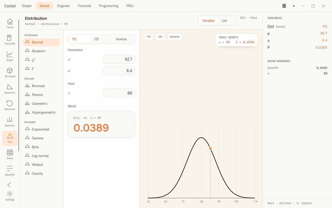
Open the Dist tile on the School apps rail. The window has three columns: a distribution picker on the left, an inputs and result column in the middle, and a large graph on the right that draws the curve or bars and shades the area you ask about. A right-hand panel mirrors your variables and working.
Choosing a distribution. The picker lists the distributions in three groups. Continuous distributions carry a small curve glyph; discrete ones carry a bars glyph.
| Group | Distributions |
|---|---|
| Continuous | Normal, Student-t, χ² (chi-square), F |
| Discrete | Binomial, Poisson, Geometric, Hypergeometric |
| Extended | Exponential, Gamma, Beta, Log-normal, Weibull, Cauchy |
Pick one and its parameters appear in the middle column, each with its label and a starting value - μ and σ for Normal, n and p for Binomial, df (degrees of freedom) for Student-t and χ², and so on. Edit a parameter and the graph redraws at once.
Choosing the form. Above the parameters is a three-way toggle: PD, CD, and Inverse. This is where you tell Castiel which of the three questions above you are asking. The form you pick changes the input fields below the parameters:
| Form | What it asks | Input fields |
|---|---|---|
PD |
Density (continuous) or mass (discrete) at one point | a single point - x for continuous, k for discrete |
CD |
Cumulative probability across a range | a Lower bound and an Upper bound, giving P(a ≤ X ≤ b) |
Inverse |
The value (percentile) for a given probability | a probability p, between 0 and 1 |
Variable or List. A toggle in the header switches between Variable input - one typed point, the usual case - and List input, which runs a whole column of values through the same distribution and returns a table of results. The examples below use Variable input.
Reading the result. The middle column shows the answer in a result card; for a CD query on a continuous distribution the graph shades the region between your two bounds and prints the area - the probability - beneath it. If a parameter is out of range (for example a negative standard deviation, or a binomial p above 1), the field is ringed and a short note explains the problem rather than returning a meaningless number.
Worked example 1 - a normal probability between two bounds
A machine fills bottles to a mean of μ = 500 ml with a standard deviation of σ = 5 ml, and the fill is normally distributed. What is the probability that a bottle holds between 495 ml and 505 ml - that is, within one standard deviation of the target?
This is a cumulative question over a range, so it is a CD query.
- In the picker, choose Normal (in the Continuous group).
- Set the parameters:
μto500,σto5. - Set the form toggle to
CD. - In the input fields, type
495intoLowerand505intoUpper. - Read the result. The graph shades the band between 495 and 505, and the area works out to about 0.6827 - roughly a 68 percent chance.
That number is the 68-95-99.7 rule in action: 495 to 505 is exactly μ ± σ, and about 68 percent of a normal distribution lies within one standard deviation of its mean. Widen the bounds to 490 and 510 (that is μ ± 2σ) and the area grows to about 0.9545 - the 95 in the rule.
Worked example 2 - a binomial probability
A fair coin is tossed 20 times. What is the probability of getting exactly 10 heads?
Counting successes in a fixed number of independent, equal-chance trials is binomial, with n = 20 and p = 0.5. "Exactly 10" asks for the probability mass at a single count, so it is a PD query.
- In the picker, choose Binomial (in the Discrete group). The graph switches to bars.
- Set the parameters:
nto20,pto0.5. - Set the form toggle to
PD. - Type
10into the point field (labelledkfor a discrete distribution). - Read the result: about 0.1762, so roughly a 17.6 percent chance of exactly 10 heads.
Notice that even the single most likely count happens less than a fifth of the time - with 21 possible outcomes (0 through 20 heads), the probability is spread across all of them. To ask a range question instead, such as "10 or more heads," switch to CD and set the bounds to cover counts from 10 upward; the app sums the bars in that range for you.
A note on the other distributions
The same three forms - PD, CD, Inverse - work identically for every distribution in the picker. Student-t, χ², and F are continuous distributions used in hypothesis testing and appear when you compare samples or test a claim; each is shaped by its degrees of freedom (df). Poisson counts how many rare events occur in a fixed interval; Geometric counts trials until the first success; Hypergeometric models drawing without replacement. The Extended group adds further continuous families for engineering and modelling work. Whichever you pick, the workflow is the same: set the parameters, choose the form, type your point, bounds, or probability, and read the area.
See also
- Distributions (School) - the full guide to the Distributions app surface.
- Statistics basics - mean, standard deviation, and summarising data.
- Probability simulation - dice, coins, and spinners that generate random outcomes to explore.
- Number theory - factorials and combinations, the counting behind the binomial distribution.