The School graph

The School graph is where you plot functions and read them as pictures and as tables of numbers. You reach it from the Graph tile on the left apps rail, one step below Calculate. Use it whenever you want to see a function rather than evaluate it at a single point: to watch how x² − 2 dips below the axis and climbs back, to compare two curves at once, to find where a curve crosses zero, or to read a neat column of x and y values.

It plots ordinary functions of x — you write the right-hand side of y = and the curve appears. For everyday single-answer arithmetic use the School calculator; for surfaces z = f(x, y) use the 3D Graph. See the School apps for the full rail.

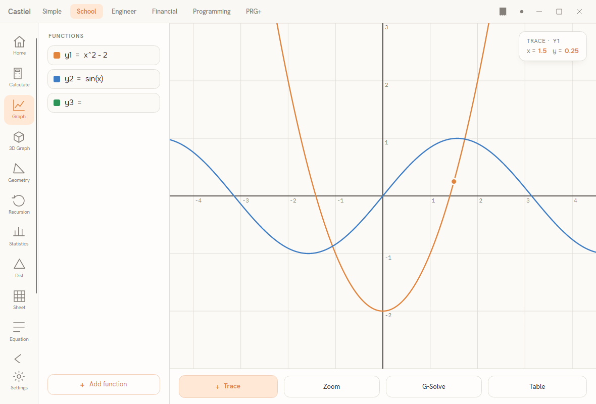
The window has three parts. Down the left is the apps rail (Home, Calculate, Graph, 3D Graph, Geometry, Recursion, Statistics, Dist, Sheet, Equation, Settings). Next to it is the function panel, a 260-pixel column headed FUNCTIONS that holds your list of y = expressions. The rest of the window is the plot canvas, with a four-button toolbar — Trace, Zoom, G-Solve, Table — pinned along the bottom. A small readout card appears over the top-right of the canvas while you trace, and the canvas swaps to a table when you choose Table.

Entering functions

Each row in the function panel is one function to plot. A row has three parts, left to right: a small colour swatch that keys the row to its curve, a y label (y1, y2, y3, ...), and an editable expression box for the right-hand side.

Type a function. Click into a row's expression box and type the formula in terms of x, exactly as you would type it in the calculator's linear entry — x^2 - 2, sin(x), 2*x + 1. The curve is drawn as soon as the expression is valid; there is no separate "plot" button. In the screenshot y1 is x^2 - 2 and y2 is sin(x), and both are already on the canvas.

More than one function. The panel starts with three rows, and each keeps its own colour so you can tell the curves apart. The colours follow a fixed order: y1 is the warm accent, y2 is blue, y3 is green, then the sequence repeats for further rows. The fourth curve onward is drawn with a dashed line so a repeated colour is still distinguishable at a glance. The swatch beside each row always matches the colour of that row's curve.

Add and clear. Press + Add function at the foot of the panel to append a fresh empty row with the next colour. An empty row is simply inert — it draws nothing — so the quickest way to take a curve off the canvas is to clear its expression box; the other curves are untouched. Type a formula back in and the curve returns.

When an expression will not parse. If what you type is not a valid formula, the row marks itself as being in error and no curve is drawn for it, while the other rows keep working. Correct the text and the error clears. An empty row is never an error; it is just waiting for input.

A note on trigonometry: a function such as sin(x) is plotted using School mode's current angle mode, the same RAD / DEG / GRA setting the calculator uses. The default is radians, which is why the sine wave in the screenshot completes one full ripple every 2π (about 6.28) along the x-axis. See Trigonometry for what the angle mode changes.

Reading the plot

The canvas draws a warm grid with the two heavy axis lines — the vertical y-axis at x = 0 and the horizontal x-axis at y = 0 — and numeric labels along the gridlines. The grid spacing chooses round steps (1, 2, 5, and their tens) and re-labels itself as you zoom, so the numbers stay readable at any scale.

Each curve is drawn in its row's colour. In the screenshot the orange parabola is y1 = x² − 2 (its lowest point sits at y = −2, where the formula bottoms out) and the blue wave is y2 = sin(x). Where a function is undefined the curve simply breaks rather than drawing a false vertical jump across the gap.

The view and analysis tools

The four toolbar buttons choose what a click or drag on the canvas does. The active tool is highlighted; in the screenshot Trace is lit. Zoom and the mouse wheel reshape the view; Trace, G-Solve, and Table read values off the curves.

Zoom. Two ways to change how much of the plane you see:

• The mouse wheel always zooms, whichever tool is active: roll up to zoom in, down to zoom out, centred on the pointer. On a touch screen, pinch to zoom the same way.
• Select Zoom and drag a box across the canvas; releasing zooms the view to fit the box you drew. This is the way to frame a specific region tightly.

Trace. Select Trace, then press and drag across the canvas. A dot rides the nearest curve and follows it as you move sideways, and a trace card appears at the top-right of the canvas reading the curve's name and the coordinates under the dot — TRACE · Y1, then x = and y =. In the screenshot the dot sits on the parabola at x = 1.5, y = 0.25. The y value is a real evaluation of the function at that x, not a pixel estimate, so the readout is exact to the displayed digits. Drag onto a different curve and the trace snaps to whichever curve is nearest the pointer, updating the card's Y label to match.

G-Solve. Select G-Solve to open a small panel of analysis actions with a status line beneath them. Each acts on the functions currently on the canvas and marks its answer with a labelled dot:

Because these tools work over the visible range, pan or zoom so the feature you want is on screen before you press the button — a root off the side of the current view is reported as not found until you bring it into frame.

Table. Select Table to dock a value table over the right of the canvas. It tabulates the first plotted function across the visible x-range in two columns, x and y. A step control at the top sets the spacing between rows (down to 0.05); lower it for a finer table, raise it for a coarser one. The table refreshes as you change the step or edit the function, and where the function is undefined at a given x the y cell shows a dash (—). Scroll the panel to run down the list.

A worked example

Plot a parabola, read a point off it, confirm that point in the table, and find the root.

1. On the Graph tile, click the first row's expression box and type x^2 - 2. The orange curve appears — a parabola whose lowest point is at y = −2.
2. Select Trace and drag the dot along the curve until the trace card reads x = 1.5. The card shows y = 0.25 — because 1.5² − 2 = 0.25. You have read a point off the graph without any arithmetic.
3. Select Table. With the step at 0.5, the x column steps ..., 1, 1.5, 2, ... and the y column shows 0.25 at x = 1.5 and 2 at x = 2 — the same values the curve carries, now as exact numbers you can copy down.
4. Select G-Solve and press Root. The status line reports Root: x = 1.41421356 and drops a marker where the parabola crosses the axis — the positive square root of 2, found straight off the graph.

Change the formula in the row and every reading above updates: the curve redraws, the table refills, and the next trace or G-Solve acts on the new function.

How the graph relates to the calculator and the tape

The graph and the calculator speak the same language. An expression that plots here — x^2 - 2, sin(x) — is the same formula the School calculator evaluates, so you can prototype a function in one surface and use it in the other.

The graph is a workspace for exploring, not a log: it has no Show working panel of its own, and reading a value with Trace, Table, or G-Solve does not by itself write to the shared paper tape. When you want a value committed to your worked record, take the number you read here — the traced y, a tabulated value, a root such as 1.41421356 — over to the calculator and evaluate it there; pressing EXE commits it to the tape like any other step. For how the tape itself works, see the paper tape.

Related chapters

• The School calculator — evaluating the same expressions you plot here.
• 3D Graph — plotting surfaces z = f(x, y).
• Trigonometry — the functions behind curves like sin(x), and the angle modes that shape them.
• The School apps — Statistics, Equation, Sheet, and the rest of the rail.
• The paper tape — the shared record that runs through every mode.