Chapters
The School Distributions app
The Distributions app is Castiel's probability-distribution workbench. You reach it from the Dist tile on the left apps rail, and it is where School-mode probability work lives: pick a distribution, set its parameters, and read off a probability, a cumulative area, or the value that a given probability points back to. It is the surface you use for questions like "what fraction of results fall below 80?", "how likely are exactly 3 successes in 20 trials?", and "what mark separates the top 5%?"
Use Distributions whenever the answer you want is a probability from a named distribution -- the normal bell curve, the binomial count of successes, the Poisson count of events, and eleven more. For summarising a data set (mean, standard deviation, regression), use the Statistics app instead; the two share the same lists and work well together. See the School apps for the full rail.
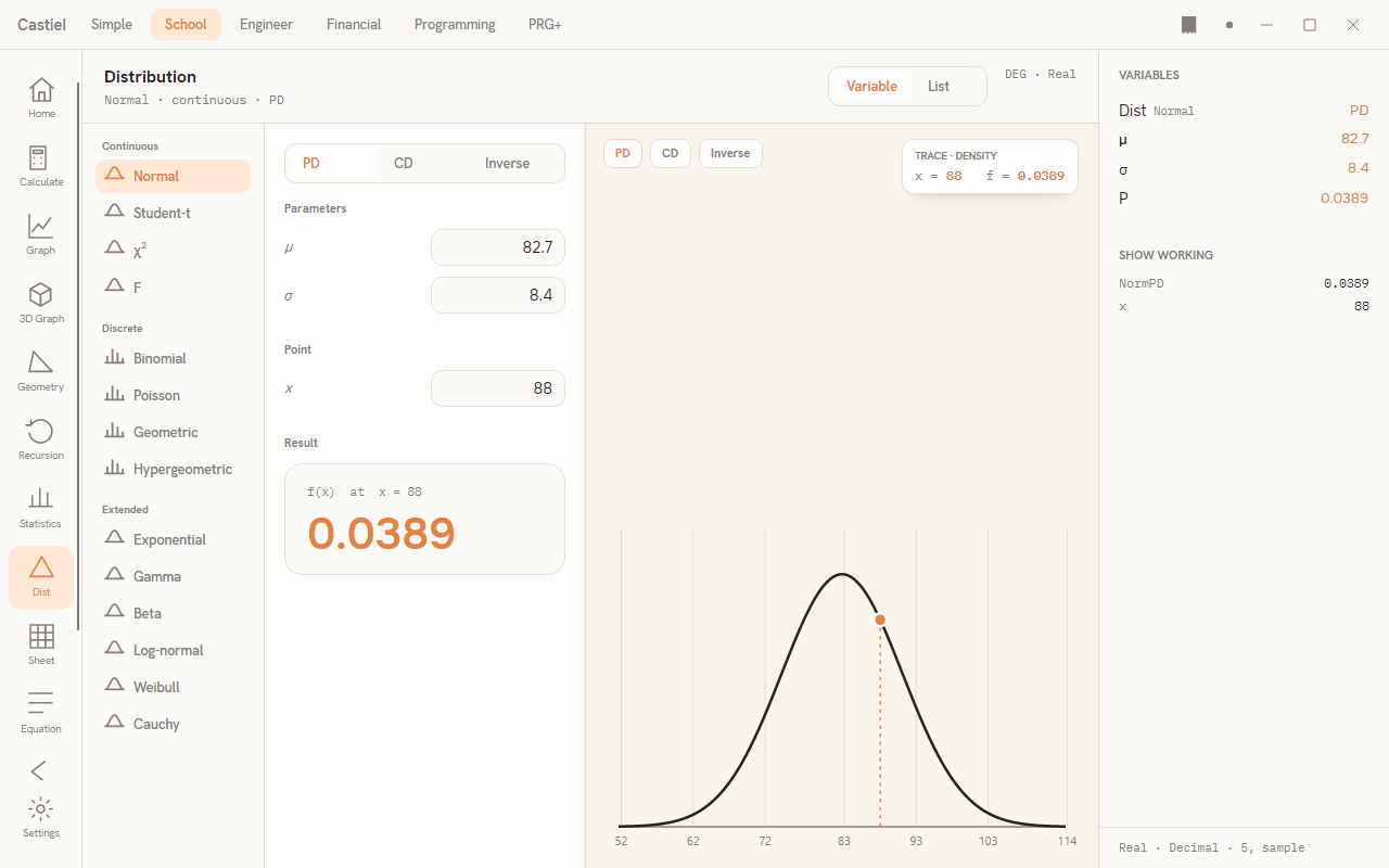
The window has three columns inside the School shell. On the left of the centre workspace is the distribution picker, grouped into Continuous, Discrete, and Extended. In the middle is the input column: the PD/CD/Inverse form toggle, the parameter fields, the point or bound inputs, and the result. Filling the right of the workspace is the graph, a large plot of the chosen distribution with the current calculation drawn on it. Down the far right is the shared Variables / Show working panel, which mirrors the calculation into the paper tape.
Choosing a distribution
The picker lists fourteen distributions in three groups. A small glyph beside each name marks its shape: a smooth curve for continuous distributions (any value in a range) and a bar chart for discrete ones (whole-number counts). Select one and its parameter fields rebuild beneath the form toggle.
| Group | Distributions | Parameters |
|---|---|---|
| Continuous | Normal | μ (mean), σ (standard deviation) |
| Student-t | df (degrees of freedom) |
|
| χ² (chi-squared) | df |
|
| F | df₁, df₂ |
|
| Discrete | Binomial | n (trials), p (success probability) |
| Poisson | λ (mean rate) |
|
| Geometric | p |
|
| Hypergeometric | n, M, N |
|
| Extended | Exponential | λ (rate) |
| Gamma | α (shape), β (rate) |
|
| Beta | α, β |
|
| Log-normal | μ, σ |
|
| Weibull | k (shape), λ (scale) |
|
| Cauchy | x₀ (location), γ (scale) |
The eight Continuous and Discrete distributions are the standard School set; the six in the Extended group are Castiel additions for work that goes beyond the basics. Every distribution is available in all three calculation forms below.
Parameters. Type each parameter into its field on the right of the label. The graph and the result update as you type. Parameters have natural limits: a standard deviation, rate, shape, or scale must be greater than 0, and any parameter that is itself a probability (p) must lie between 0 and 1. If you enter a value outside its range, the field gets a warning ring and the result area explains what is wrong (see When a value is out of range below). The curve is still drawn from the last valid parameters, so the picture never disappears while you correct a typo.
PD, CD, and Inverse
The three-way toggle at the top of the input column chooses what you are calculating. The same toggle appears as a badge on the top-left of the graph so you can always see which mode is drawn.
PD -- probability density (or mass). PD asks about a single point. Enter one value in the Point field:
- For a continuous distribution the field is labelled
x, and the result is the densityf(x)-- the height of the curve atx. Density is not itself a probability; it is the curve's value at that point, and probabilities come from areas under it. - For a discrete distribution the field is labelled
k, and the result isP(X = k)-- the exact probability of that whole-number outcome. This is a genuine probability between 0 and 1.
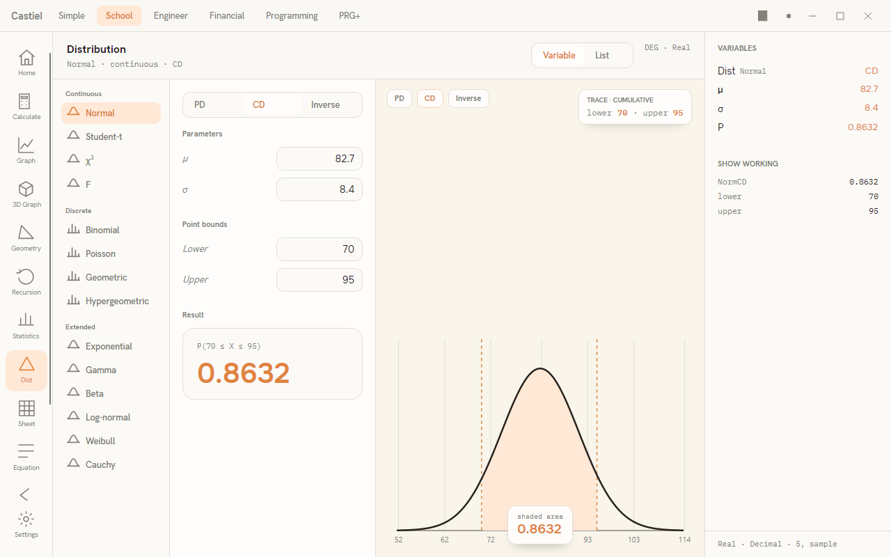
CD -- cumulative. CD asks about a range. Enter a Lower and an Upper bound, and the result is the probability of landing between them, written P(a ≤ X ≤ b). This is the shaded area under the curve (or the sum of the highlighted bars for a discrete distribution). To get a one-sided "less than" probability, set the lower bound far below the distribution -- for a standard normal, a lower bound of -100 effectively means "from minus infinity", so the result is P(X ≤ b). If you enter the bounds in the wrong order, Castiel swaps them for you.
Inverse. Inverse runs a cumulative calculation backwards. Enter a Probability p between 0 and 1, and the result is the value x for which P(X ≤ x) = p -- the cut-off that puts probability p below it. This is how you find percentiles: the 95th percentile is the inverse at p = 0.95. A probability outside 0 to 1 is rejected with an explanation.
The graph reflects each mode. In CD the area between the bounds is shaded and a floating shaded area label shows its value; in Inverse the area up to the answer is shaded and labelled P(X ≤ x); in PD the single point (or bar) is marked. A trace read-off card in the top-right corner of the graph restates the current point, bounds, or boundary in words.
Reading the result and the graph
In the input column the result appears in a card below the inputs, with a label naming exactly what was computed -- f(x) at x = 1.5, P(65 ≤ X ≤ 85), or x such that P(X ≤ x) = 0.95. Until you have entered every input the form needs, the card shows a dash and a hint (for example, "enter a lower & upper bound"), so a blank result always tells you what is still missing rather than showing a misleading zero.
The graph on the right is the same distribution drawn full size, with your calculation overlaid: the curve or bars, the shaded region and its boundary lines for CD and Inverse, and the marked point for PD. The header strip above the workspace carries a one-line subline summary -- the distribution name, whether it is continuous or discrete, and the current form -- and the mode readout DEG · Real.
Single value versus list input
The Variable / List toggle in the header switches how many points you evaluate at once.
- Variable (the default) evaluates one point, one pair of bounds, or one probability -- the workflow described above, with the result shown in the card.
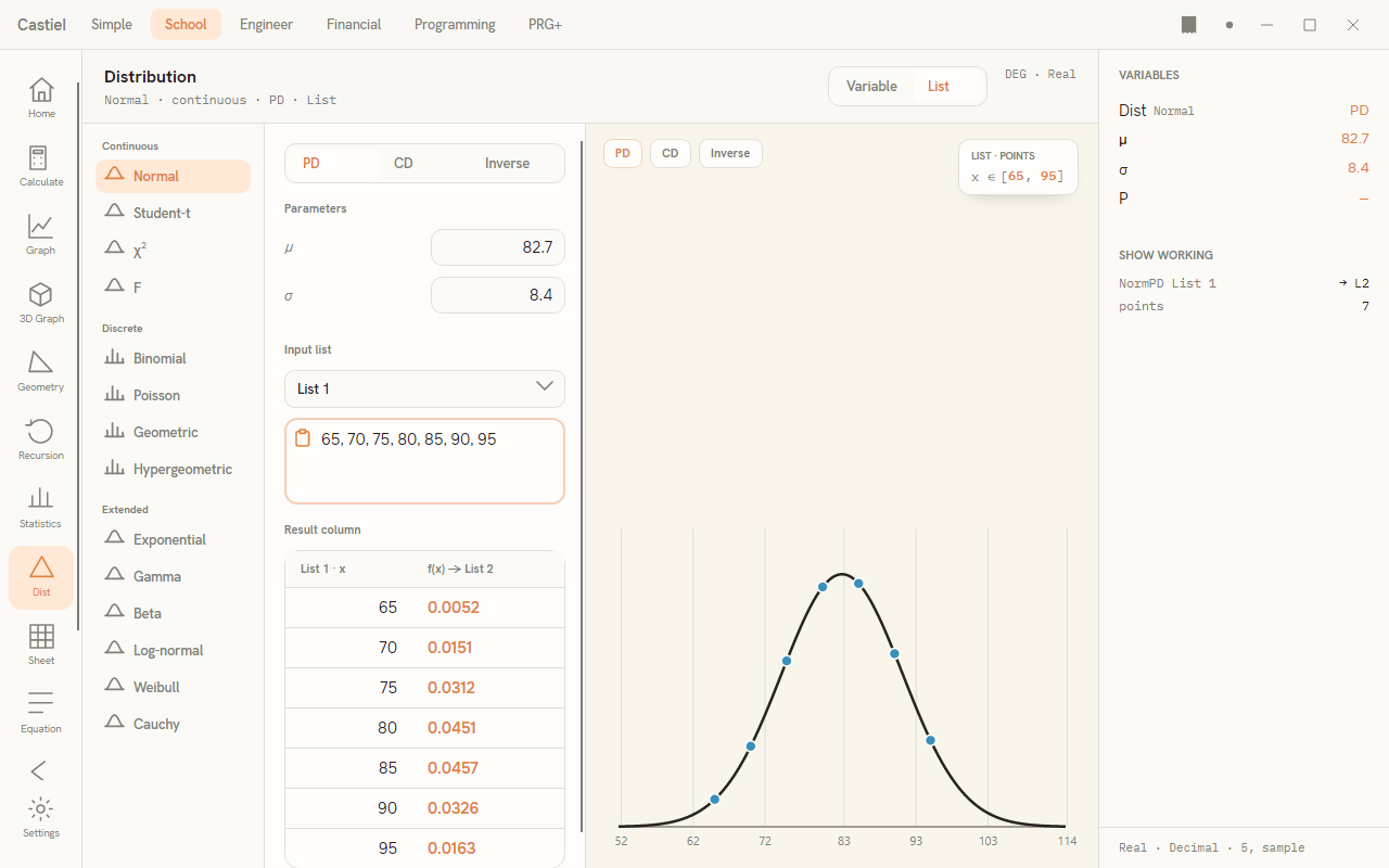
- List evaluates a whole column of values in one pass. A Paste / enter column box appears; type or paste numbers separated by commas, spaces, or new lines. Castiel evaluates the chosen form at every value and fills a two-column result table: your input value on the left, the answer on the right. The columns are labelled as
List 1in,List 2out, matching the list names in the Statistics app -- so a column of marks you built there can be run through a distribution here.
List mode always evaluates each value as a single point: PD gives the density or mass at each value, CD gives the cumulative P(X ≤ x) at each value, and Inverse treats each entry as a probability and returns its cut-off. (The two-bound range calculation is a Variable-mode feature.)
Worked example: a normal probability between two bounds
Exam marks are approximately normal with mean 78 and standard deviation 8. What fraction of students scored between 65 and 85?
- In the picker choose Normal (Continuous group).
- Set the parameters:
μ = 78,σ = 8. - Set the form toggle to CD.
- In the Point bounds section enter
Lower = 65andUpper = 85.
The result card reads P(65 ≤ X ≤ 85) with the probability -- about 0.7571, so roughly 76% of students. On the graph the bell curve is drawn with the strip between 65 and 85 shaded, dashed lines mark the two bounds, and the floating shaded area label repeats the value. To find instead the mark below which 90% of students fall, switch to Inverse and enter p = 0.9: the answer is about 88.25.
Worked example: an exact binomial probability
A quiz has 20 true/false questions answered by guessing, so each has success probability 0.5. What is the probability of getting exactly 12 right?
- In the picker choose Binomial (Discrete group).
- Set the parameters:
n = 20,p = 0.5. - Set the form toggle to PD.
- In the Point section enter
k = 12.
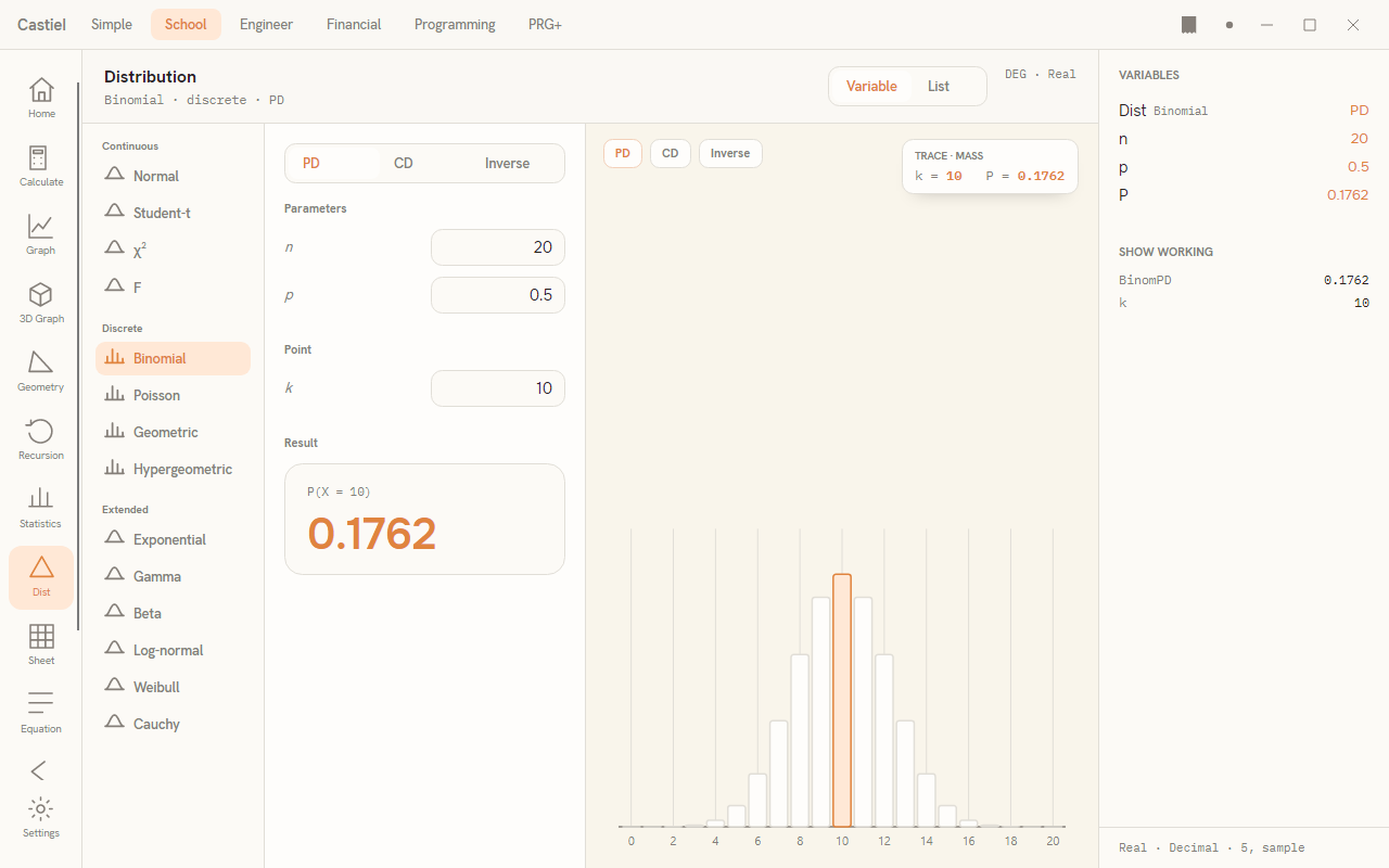
The result card reads P(X = 12) with the value -- about 0.1201. The graph shows the binomial as a row of bars, with the bar at k = 12 highlighted. To ask instead "12 or more correct", switch to CD and enter Lower = 12, Upper = 20; Castiel sums the bars from 12 to 20 inclusive and shades them.
When a value is out of range
Distributions have domains, and Castiel guards them rather than returning a meaningless number. If you enter a parameter outside its allowed range -- a standard deviation of 0, a negative rate, a probability above 1 -- the offending field gains a red warning ring and the result area becomes a note that names the field, explains the limit in plain terms, and shows the bad value. The graph keeps drawing the curve from the last valid parameters so you keep your bearings while you fix the entry. The same guard covers the Inverse form: a probability p must be between 0 and 1, and anything else is flagged before it is evaluated.
Variables, Show working, and the paper tape
The right-hand panel has two parts. Variables lists the current distribution, each parameter and its value, and the result (P for a probability, x for an inverse) -- a compact summary of the whole calculation. Show working below it is a mini-tape: the distribution-and-form shorthand (such as NormCD or BinomPD), the inputs you supplied, and the answer, so a completed calculation reads back as a single worked step. In List mode it records the operation against List 1 and the number of points.
This panel is a view of the same shared paper tape that runs through every School app, filtered to your Distributions steps. Because the tape keeps its history, you can scroll back through a sequence of probability calculations, and the results carry across to other apps -- most usefully, a List-mode result column lands in List 2 for the Statistics app to chart or summarise. For the full behaviour of the tape -- editing, correcting, and exporting -- see the paper tape.
Related chapters
- Probability distributions -- the mathematics behind each distribution, and when to reach for which.
- Statistics -- summarising data and sharing the
List 1/List 2columns with this app. - The School apps -- Calculate, Graph, Equation, and the rest of the rail.
- The paper tape -- reviewing, correcting, and exporting your working.